A. Introduction

Speaker verification is the task that given two segments of audio signal, we are supposed to verify whether both signals came from the same identity of the speaker or not. While inferencing, we first transform the audio signal into the corresponding speaker embedding, then calculate the similarity between two embeddings which is used to compare with the certain threshold later.

Speaker Retrieval is the task that given a paragraph of audio content, usually long, and a segment of audio represented one specific speaker identity as the input, we have to precisely point out the corresponding parts in the audio paragraph which owns the same identity as the input signal. In our experiment setting, we construct a pool set which includes a plenty of voice segments of several speakers, along with a target set which is composed of voice segments of speakers same as those in the pool set, each speaker has one corresponding segment within the target set.

In this article, we will first introduce the results of the speaker verification task and several skills to improve the performance, then show a new method that add a quantization part in the loss function, in order to fasten the process and reduce the memory usage in the speaker retrieval task.

B. Speaker Verification

First, we utilize four different speaker embedding models [1][2][3][4] on three datasets [5][6][7] and evaluate the performance of the results through two metrics. Also note that pyannote.audio (pyannote) and Efficient-TDNN (sugar) are both pretrained on the voxceleb dataset, while ECAPA-TDNN (spkrec) is pretrained on the cnceleb dataset.

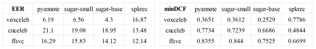
In the result, we can quickly observe that the language information somehow makes an impact on the performance of the speaker verification task. To alleviate such influence, we implement several skills toward the speaker embeddings generated from the pre-trained models, including the concatenation and domain adaptation.

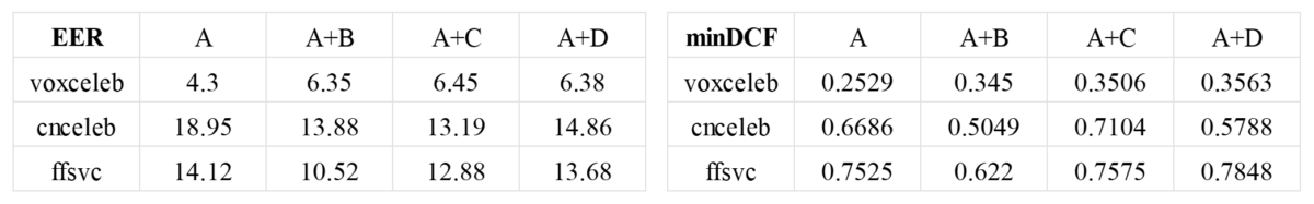
The table below shows the speaker verification results generating from the concatenated embeddings. The corresponding models are pretrained Efficient-TDNN (A), pretrained ECAPA-TDNN (B), Efficient-TDNN trained on cnceleb for 12 epochs (C), and Efficient-TDNN trained on cnceleb for 64 epochs (D).

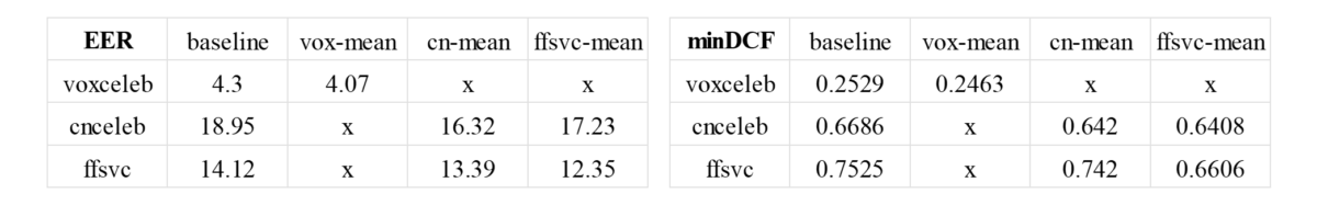
To realize the domain adaptation [8], we subtract the mean of the whole dataset from each embedding before the comparison. This also works even when the dataset that used to generate the mean is different from the target dataset.

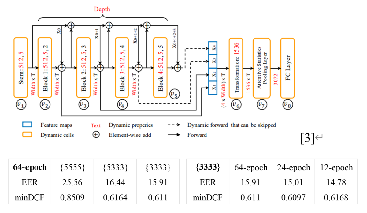
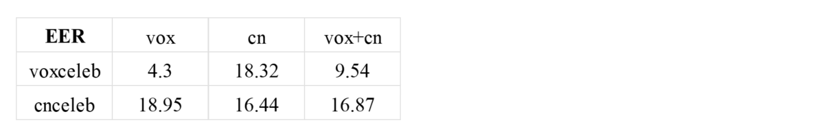
Also, since we are more interested in the performance on Chinese datasets, we train the Efficient-TDNN, which is three times smaller than the ECAPA-TDNN, with the cnceleb dataset. What’s more, we further train the Efficient-TDNN with both voxceleb and cnceleb datasets to see whether such model has the ability to handle both languages itself.

The table below shows the results on the cnceleb dataset by using the embeddings from the Efficient-TDNN trained with such dataset under dynamic architectures and different training epochs. We list the results of training the Efficient-TDNN model with both voxceleb and cnceleb datasets, too.

C. Speaker Retrieval

When it comes to details of the new-added quantization part, the overall loss function can be separated into two terms. The first term is the cross-entropy loss for the classification during training, and the second term is the L2 loss, which is added as a quantization loss. The target of the L2 loss is the integer 1 or -1, which forces the content of embeddings to be as close to 1 or -1 as they can, thus leads to a smaller influence while directly clamping them to 1 and -1. [9][10]

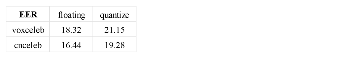
We use only the cnceleb dataset to fine-tune the Efficient-TDNN and starts from the checkpoint which has trained 64 epochs on the very model and dataset, but with the original loss function. First, we show the result on the speaker verification task.

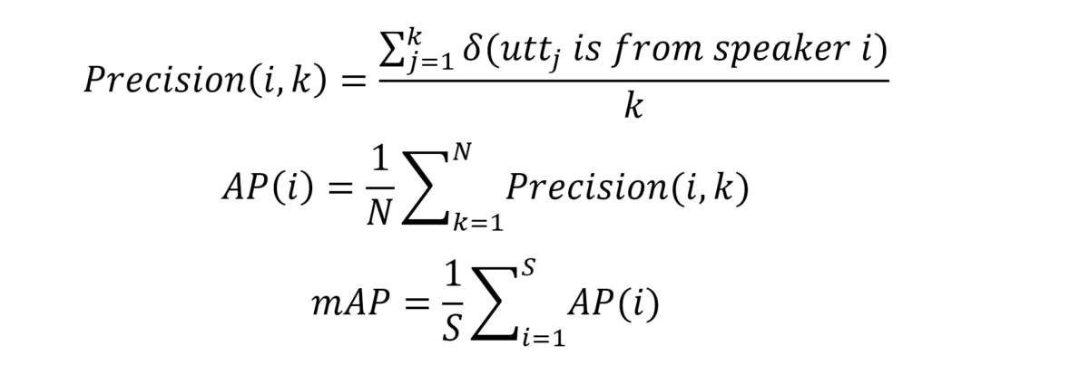
For the speaker retrieval task, we utilize three different architectures to generate embeddings and inference on three datasets. The metric to evaluate the performance is mAP, which is defined as:

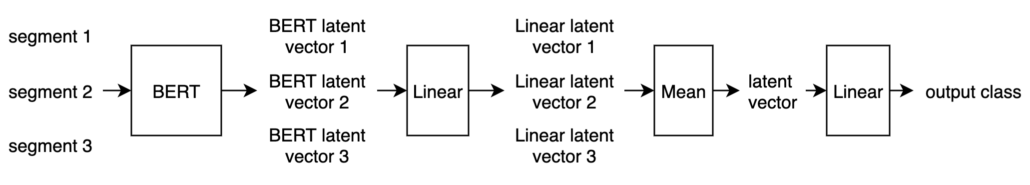
The detailed of three architectures are listed below. The first architecture is composed by HuBERT, an SSL model, followed with an additional linear layer, and a hyperbolic tangent layer. [11] The output of the hyperbolic tangent layer then uses to calculate the L2 quantization loss and used to calculate the cross-entropy loss after passing another linear layer. The second architecture uses the fine-tuned Efficient-TDNN mentioned above rather than the SSL model. Though the third architecture seems to be similar to the second one, it uses the 64-epoch pretrained model with the original loss function and thus generating floating number embeddings as a baseline for the quantization method. Note that the first architecture is trained on the voxceleb1 dataset while the other two are trained on the cnceleb dataset.

After the embeddings are generated, there are two ways for us to calculate distances between voice segments in the target set and those in the pool set, cosine distance for embeddings with floating numbers and hamming distance for those with quantized numbers. For the number of files in the pool set, we choose 10 files for each speaker in voxceleb2 and cnceleb datasets and choose all of the files in the voxceleb1 dataset. The experiment result is shown as below.

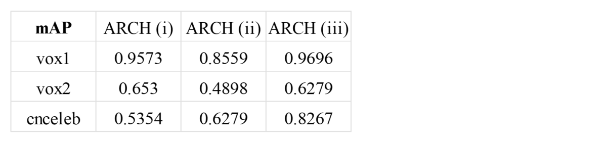
Despite that the performance of the quantization method has an approximately 11%~14% decrease compared to the baseline, the computation speed can gain a nearly 60% increase while calculating the distance and comparing through the pool set. What’s more, the memory usage can be significantly reduced, since a k-bit floating number requires k times of storage spaces than a boolean number.

D. Reference

[1]     pyannote.audio: neural building blocks for speaker diarization

https://arxiv.org/abs/1911.01255

[2]     A Comparison of Metric Learning Loss Functions for End-To-End Speaker Verification

https://arxiv.org/abs/2003.14021

[3]     EfficientTDNN: Efficient Architecture Search for Speaker Recognition

https://arxiv.org/abs/2103.13581

[4]     SpeechBrain: A General-Purpose Speech Toolkit

https://arxiv.org/abs/2106.04624

[5]     VoxCeleb: a large-scale speaker identification dataset

https://arxiv.org/abs/1706.08612

[6]     CN-CELEB: a challenging Chinese speaker recognition dataset

https://arxiv.org/abs/1911.01799

[7]     FFSVC

FFSVC 2022

[8]     The SpeakIn System for Far-Field Speaker Verification Challenge 2022

speakin_22.pdf (ffsvc.github.io)

[9]     Scalable Identity-Oriented Speech Retrieval

Scalable Identity-Oriented Speech Retrieval | IEEE Journals & Magazine | IEEE Xplore

[10]   Deep Hashing for Speaker Identification and Retrieval

INTERSPEECH19_DAMH.pdf (jiangqy.github.io)

[11]    Why does Self-Supervised Learning for Speech Recognition Benefit Speaker Recognition?

[2204.12765] Why does Self-Supervised Learning for Speech Recognition Benefit Speaker Recognition? (arxiv.org)

Taiwan has four important upcoming referendums on December 18, 2021. “Pork Imports”, “Referendum Dates”, “Nuclear Plant”, “Algae Reef Protection.” According to previous research, disinformation and manipulation of the media could influence public opinion on topics like these referendums. This study will examine how Facebook has affected the polarization of public opinion on these topics over the previous eleven months. The phenomenon of public opinion polarization and the factors affecting policy support and political attitudes will be analyzed using artificial intelligence technology. The polarization impact of pages that demonstrated evidence of potential media manipulation through coordinated behavior were considered. Within these pages, those that were shared most often are referred to as “amplifiers.”

FB_Research_Project

Introduction

Speaker Diarization is the task to partition audio recordings into segments corresponding to the identity of the speaker. In short, a task to identify “who spoke when”. Speaker diarization can be used to analyze audio data in various scenarios, such as business meetings, court proceedings, online videos, just to name a few. However, it is also a very challenging task since characteristics of several speakers have to be jointly modelled.

Traditionally, a diarization system is a combination of multiple, independent sub-modules, which are optimized individually. Recently, end-to-end deep learning methods are becoming more popular. The metric for speaker diarization is diarization error rate (DER), which is the sum of false alarm, missed detection and confusion between speaker labels.

In this article, we will introduce our upcoming speaker diarization system first, then give an overview of the latest research in end-to-end speaker diarization.

Our Method

Our product uses a traditional diarization pipeline, which consists of several components: speech turn segmentation, speaker embedding extraction, and clustering. We utilize pyannote.audio [2], an open-source toolkit for speaker diarization, to train most of our models. 

1. Speech Turn Segmentation

The first step of our diarization system is to partition the audio recordings into possible speaker turn segments. A voice activity detection model is used to detect speech regions, while removing non-speech parts. Speaker change detection model is used to detect speaker change points in the audio. Each of these models are trained to optimize a sequence labeling task: With sequence of audio features as input, output a sequence of labels.

For both models, there are some tunable hyperparameters which determine how sensitive the models are on segmenting the audio. For the speaker change detection model, only audio frames with detection score higher than the threshold “alpha” are marked as speaker change points. We notice that it is generally more beneficial to segment more aggressively (i.e. split the whole audio into more segments) in the speech turn segmentation stage, so as to make sure most segments only contain one speaker. After the clustering stage, we can merge segments assigned to the same speaker for better Speech Recognition performance in following stages.

2. Speaker Embedding Extraction

After performing speech turn segmentation, in order to facilitate clustering of speaker segments in the clustering module, a speaker embedding model is used to obtain a compact, fine-grained representation for each segment.

The model we choose is SincTDNN which is basically a x-vector architecture where filters are learned instead of being handcrafted. Additive angular margin loss is applied to train the model. 

We utilize CNCELEB [3], an open source large-scale chinese speaker recognition dataset, to fine tune the model pretrained on voxceleb. CNCELEB is a challenging, multi-domain dataset consisting of 3,000 speakers in 11 different genres. By using such a diverse dataset, we expect our model to be stable enough when facing various real life scenarios. We also notice that only very few epoch is needed to fine tune the model, and that speaker embedding with lower EER may not always imply lower diarization error rate.

3. Clustering

Traditional cluster methods can be used to cluster the speaker embedding, identifying which speaker each segment belongs to. In our system, we leverage affinity propagation for short audio, and KMeans for long audio. Since we do not know how many speakers are in the recording, affinity propagation has relatively better performance than KMeans as it can determine the number of clusters directly. While for KMeans, we estimate the best number of clusters by finding the elbow of derivatives in MSCD. However, we resort to KMeans instead of affinity propagation for longer audio files since affinity propagation tends to be slower in this situation.

Combining all components

With all the aforementioned components trained, we can combine them into a complete pipeline for diarization. Several hyperparameters are optimized jointly to minimize diarization error rate on a certain dataset. 

Compared to our previous system, the current system obtains around 30% DER relative improvement on our internal dataset flow-inc, which consists of a few thousands news recordings.  Most improvements stem from improved speaker embedding and clustering method, which improved from 15% to 8% DER for oracle speech turn segmentation setting.

In our production system, we also allow some extra customization for our users. For instance, if the user provides the number of speakers in the recording, we can use KMeans to recluster according to the number of speakers. Also, if the user provides or corrects some speaker labels of the utterances, this extra information is involved when updating the cluster centers. Re-cluster will progress with partial initialization based on updated centers, resulting in more accurate predictions.

Finally, the output of speaker diarization can be further fed to the input of an ASR system, and the final output is the transcript for each speaker turn. It is not very certain if diarization can help improve ASR performance; however, recent work has shown that ASR with diarization can obtain comparable WER as state-of-the-art ASR system, but with extra speaker label information.

What’s Next?

While most systems in production still follow the traditional pipeline of speech turn segmentation + clustering, End-to-end diarization systems are receiving more and more attention. As traditional pipeline assumes single-speaker per block while extracting speaker embedding, it can by no means handle the problem of overlapping speech. End-to-end diarization systems receive frame-level speech features as input, and directly output frame-level speaker activity for each speaker, thus can handle overlapping speech in an easy manner. Also, end-to-end systems minimize diarization error directly, getting rid of the need to tune hyper-parameters of several components. Today, end-to-end systems are able to perform on par with, or even better than traditional pipeline systems in many datasets.

However, end-to-end systems still have several drawbacks. Firstly, these systems cannot easily handle an arbitrary number of speakers. The originally proposed EEND [4] can only deal with a fixed number. Several follow-up works attempt to address this problem, but their systems still struggle to generalize to real world settings, where there may be more than 3 speakers.

Secondly, while end-to-end systems are optimized directly for diarization error rate, they may easily overfit to the training dataset, for instance the number of speakers, speaker characteristics, as well as background conditions. In contrast, traditional clustering-based approaches are shown to be more robust across datasets. Lastly, most end-to-end diarization systems use transformer or conformer as their core architecture. Self-attention mechanism in transformer has quadratic complexity, which hinders the model’s capability to process long utterances or meetings.

Recently, hybrid systems integrating both an end-to-end neural network and clustering are proposed [5][6], which try to take the pros of both worlds. Hybrid systems handling overlapping speech with an end-to-end network, and able to handle an arbitrary number of speakers using clustering algorithms. Also, block processing of input audio data  [5] significantly shortens the process time of long recordings. This series of research is very promising and deserves more attention.

Finally, many state-of-the-art systems still leverage simulated mixture recordings for training, then fine tune and evaluate on real dataset. This indicates the lack of large-scale real-life dataset for end-to-end training. By introducing more challenging real-life dataset, it is believed that diarization performance can be further improved. 

Conclusion

To address the challenging task of speaker diarization, we leverage a system consisting of several neural networks: speech activity detection, speaker change detection, speaker embedding, as well as clustering algorithm. While these components are trained separately, they are optimized jointly by tuning hyper-parameters. For further work, we would like to incorporate an end-to-end segmentation model to handle overlapping speech, as well as making our system more real-time.

Reference

[1] A Review of Speaker Diarization: Recent Advances with Deep Learning https://arxiv.org/abs/2101.09624 

[2] pyannote.audio: neural building blocks for speaker diarization https://arxiv.org/abs/1911.01255

[3] CN-Celeb: multi-genre speaker recognition https://arxiv.org/abs/2012.12468   

[4] End-to-End Neural Speaker Diarization with Self-attention https://arxiv.org/abs/1909.06247 

[5] Advances in integration of end-to-end neural and clustering-based diarization for real conversational speech https://arxiv.org/abs/2105.09040 

[6] Towards Neural Diarization for Unlimited Numbers of Speakers Using Global and Local Attractors  https://arxiv.org/abs/2107.01545 

[7] The yellow brick road of diarization, challenges and other neural paths https://dihardchallenge.github.io/dihard3workshop/slide/The%20yellow%20brick%20road%20of%20diarization,%20challenges%20and%20other%20neural%20paths.pdf 

At Taiwan AI Labs, we are constantly pushing the frontier of deep music generation models. In the past year, we have rolled out Guitar Transformer (blog), which can compose human-readable guitar tabs with plausible fingerings, and Compound Word Transformer (blog), which vastly accelerated model training and inference thanks to carefully re-engineered music representation. Today, proudly making its debut is MuseMorphose, our brand new model for music style transfer.

Unlike our previous works, which offered limited possibilities for user interaction, MuseMorphose is designed to extensively engage users in the machine creative process. With MuseMorphose, one may input his/her favorite song, the length of which unlimited, and set two musical style attributes, namely, rhythmic intensity and polyphony (i.e., harmonic fullness), of every bar to his/her desired level (0~7 possible). The model will then re-create the song, taking into account the user-specified sequence of bar-level style attributes.

Listening Samples

To showcase MuseMorphose’s capabilities, let us present some of its compositions first!

In the upper example, we feed the famous 8-bar theme of Mozart’s “Twinkle, Twinkle, Little Star” to the model, and ask it to generate a style-transferred version with increasing rhythmic and harmonic intensities (going up by 1 level per bar). For the next one, we choose an 8-bar excerpt from our AILabs1K7 pop song dataset (published here) and pick three drastically different style settings for MuseMorphose to wield its creativity.

Across all the samples, MuseMorphose responds precisely to the style settings. What’s more, it sticks faithfully to the musical flow of input song while adding its own creative and harmonious touches.

MuseMorphose: The Model

Now that we have had some pleasant music, it is time to delve into the technical underpinnings of MuseMorphose.

Architecture of MuseMorphose

MuseMorphose is based on two popular deep learning models for music generation: Variational Autoencoder (VAE), and Transformer. VAE (see also: MusicVAE & Attr-Aware VAE) grants users the freedom to harness the generation through operations on its learned latent space, much like we have shown in the examples; however, its RNN backbone greatly limits the length of music it can model.

Transformer (check out: Music Transformer & MuseNet), on the other hand, can generate music of up to 5 minutes long, but its conditional generation use cases remain underexplored. People could only use global condition tokens to affect a composition’s style or instrumentation, or, in some other cases, they have to supply a full melody/track for the model to come up with an accompaniment. It has not been possible to freely edit a piece according to its high-level musical flow. Therefore, we integrate the two models to construct MuseMorphose, which exhibits both of their strengths, and gets rid of their weaknesses.

In MuseMorphose, a Transformer encoder is tasked with extracting the musical skeleton of each bar in a piece as vectors (called “latent conditions” in the figure above). Then, these skeletons are concatenated with bar-level style inputs from the user, i.e., the rhythmic intensity and polyphony levels, mapped to learned embedding vectors. Finally, the concatenated conditions enter sequentially, i.e., bar by bar, into a Transformer decoder through the in-attention mechanism developed by us, to produce the style-transferred piece.

This asymmetric encoder-decoder design ensures the fine granularity of conditions, and maintains Transformer’s inherent ability to generate long sequences. Moreover, the in-attention mechanism, which injects each bar-level condition to corresponding timesteps and all layers of the Transformer decoder, is the key to effective conditioning.

Further Materials

• Paper (preprint): arxiv.org/abs/2105.04090
• Demo website: slseanwu.github.io/site-musemorphose
• Open-source code: github.com/YatingMusic/MuseMorphose

You may take a look at our paper to find more discussions on the architecture design, training objective, and evaluation. Our demo website provides even more compositions by MuseMorphose, as well as those by the baselines it outperforms, for you to listen. Want to compose some music with MuseMorphose? No problem! Just check out our open-source implementation and pre-trained checkpoint.

If you find our work exciting, and have some thoughts/suggestions about it (e.g., what other style attributes may be added to MuseMorphose), feel free to drop us a mail. We are definitely looking forward to a lively discussion.

By: Shih-Lun Wu, Yi-Hsuan Yang (Yating Music Team, Taiwan AI Labs)