Removing Objects from 360° “Stationary” Videos

Introduction

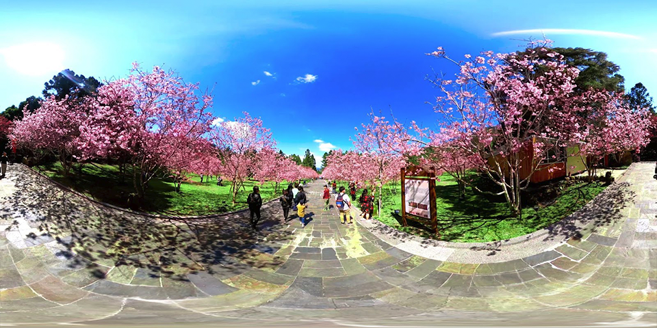
In recent years, 360° videos have become increasingly popular in providing viewers with an immersive experience where they can explore and interact with the scene. Taiwan AILabs is developing technology for the processing and streaming of 360° videos. Among the applications of our technology is Taiwan Traveler, an online tourism platform that allows visitors to experience a “virtual journey” through various tourist routes in Taiwan. A challenge we face when creating a 360° video immersive experience is the presence of cameramen in the video, which interferes with the viewing experience. Due to the fact that the 360° camera captures scenes from all possible viewing angles, the cameraman is unavoidably captured in the initial film. This article discusses a method for resolving this cameraman issue during the processing stage of 360° videos.


Cameramen Removal

Cameraman removal (CMR) is an important stage of 360° video processing, which involves masking out the cameraman and painting realistic content into the masked region. The objective of CMR is to mitigate the problem of camera equipment or cameramen interfering with the viewing experience.


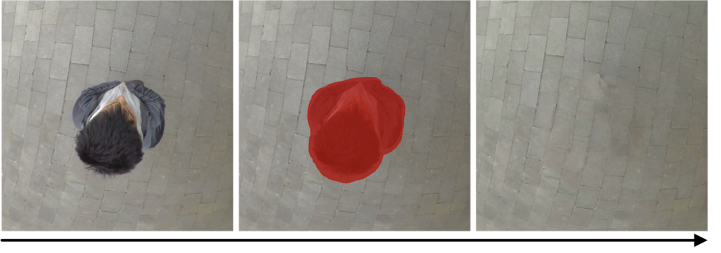
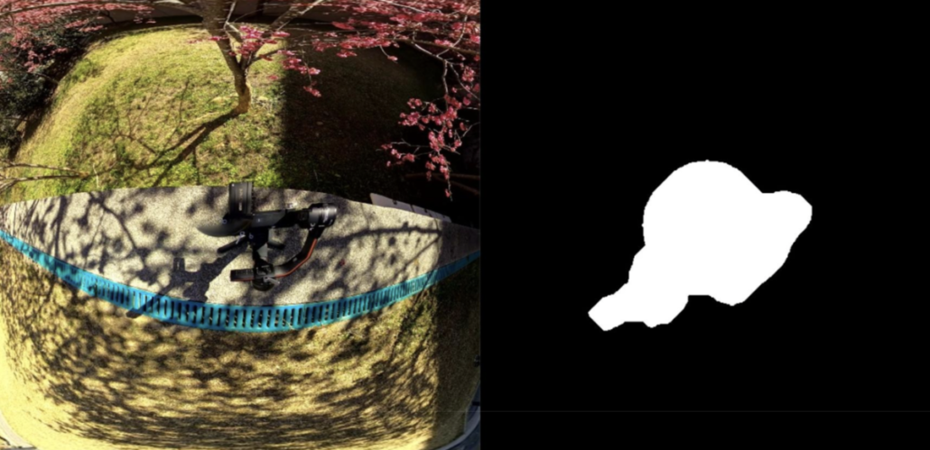
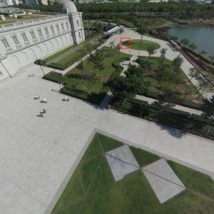
A video frame with a camera and its corresponding mask: Given a video containing a camera tripod and corresponding mask, CMR aims to “remove” the tripod by cropping the masked region and then inpainting new synthetic content therein.

In our previous blog [1] about cameraman removal, we discussed how we removed the cameraman from 8K 360° videos with a pipeline based on FGVC [2]. However, the previous method [1] is only suitable for videos taken with moving cameras. Therefore, we develop another method to remove the cameraman from stationary 360° videos.

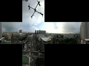
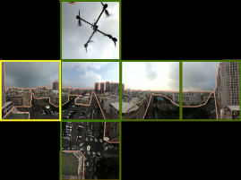
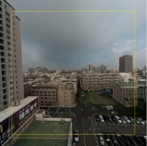
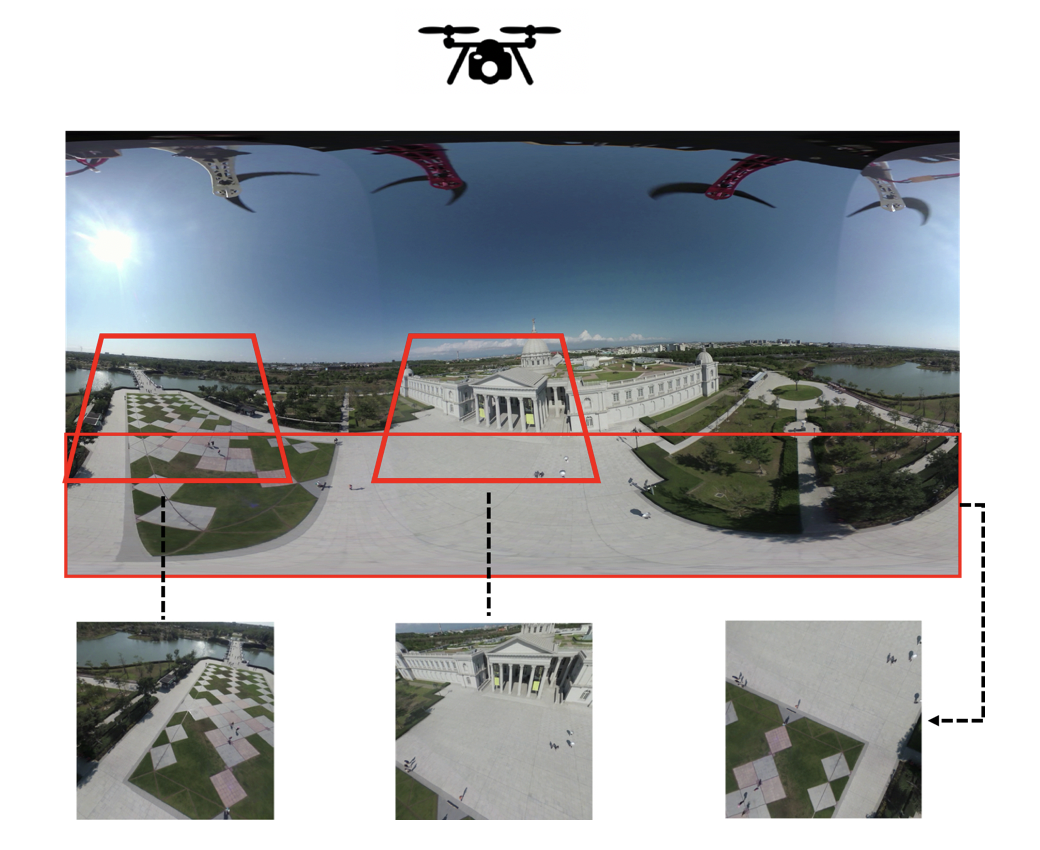
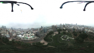
( For most of the demo videos in this blog, we do not show the full 360° video. Instead, we rotate the camera down by 90°, so that the camera points to the ground ( the direction in which the cameraman usually appears), and crop a rectangular region from the camera view. This rotation process is also present in our CMR pipeline, where we rotate the camera and crop a small region for input to the CMR algorithms. )


Stationary Video vs Dynamic Video

Before getting into the details of our stationary video inpainting method, we first discuss the difference between dynamic and stationary videos.

Dynamic videos are captured by cameras that are constantly moving. The cameraman may be walking throughout the video, for example.


Dynamic video example: a handheld video taken while walking. We want to remove the cameraman in the center.

Stationary videos, on the other hand, are filmed with little or no camera movement. As an example, a cameraman may hold the camera while staying within a relatively small area as compared to the surrounding area, or a tripod may be used to mount a camera.


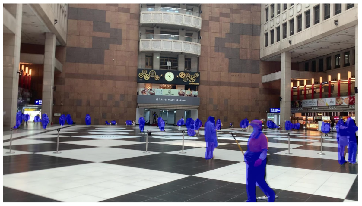
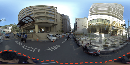
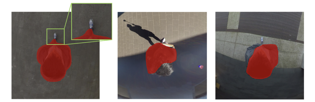
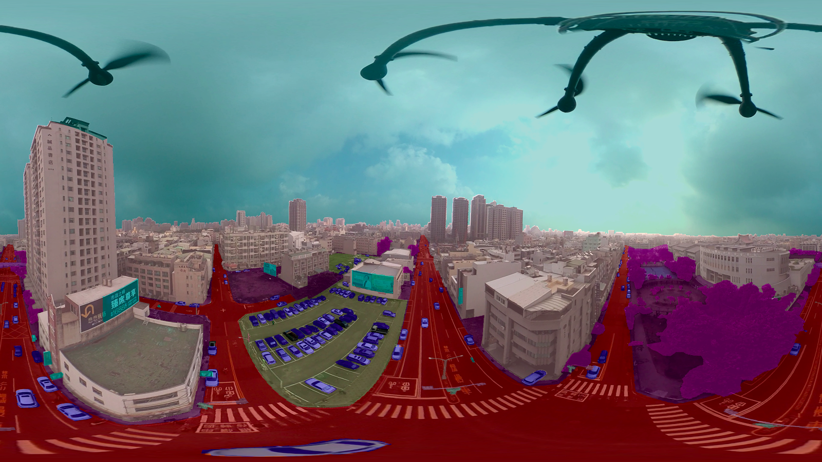
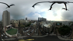
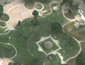
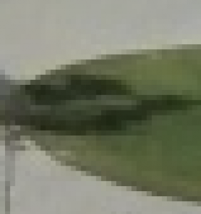
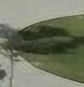
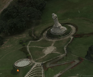
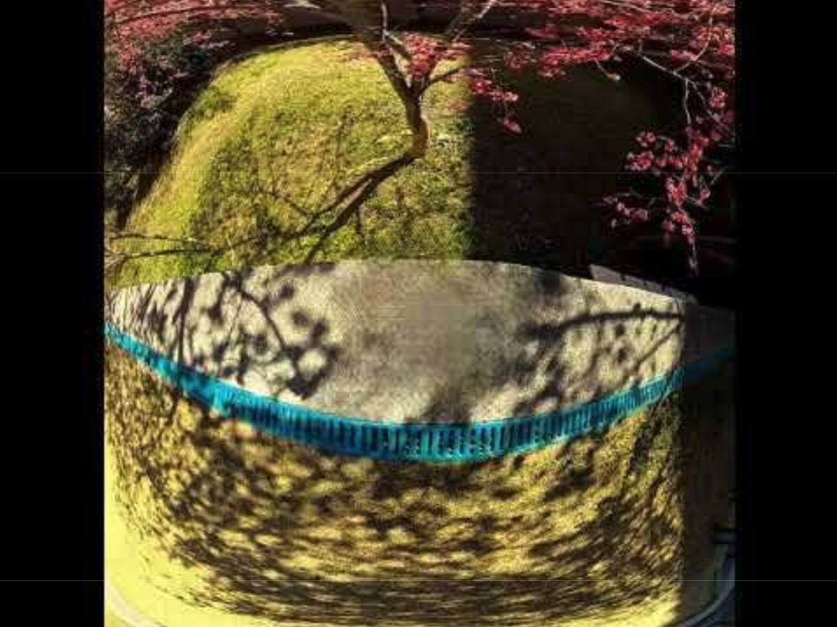
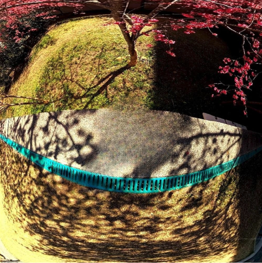
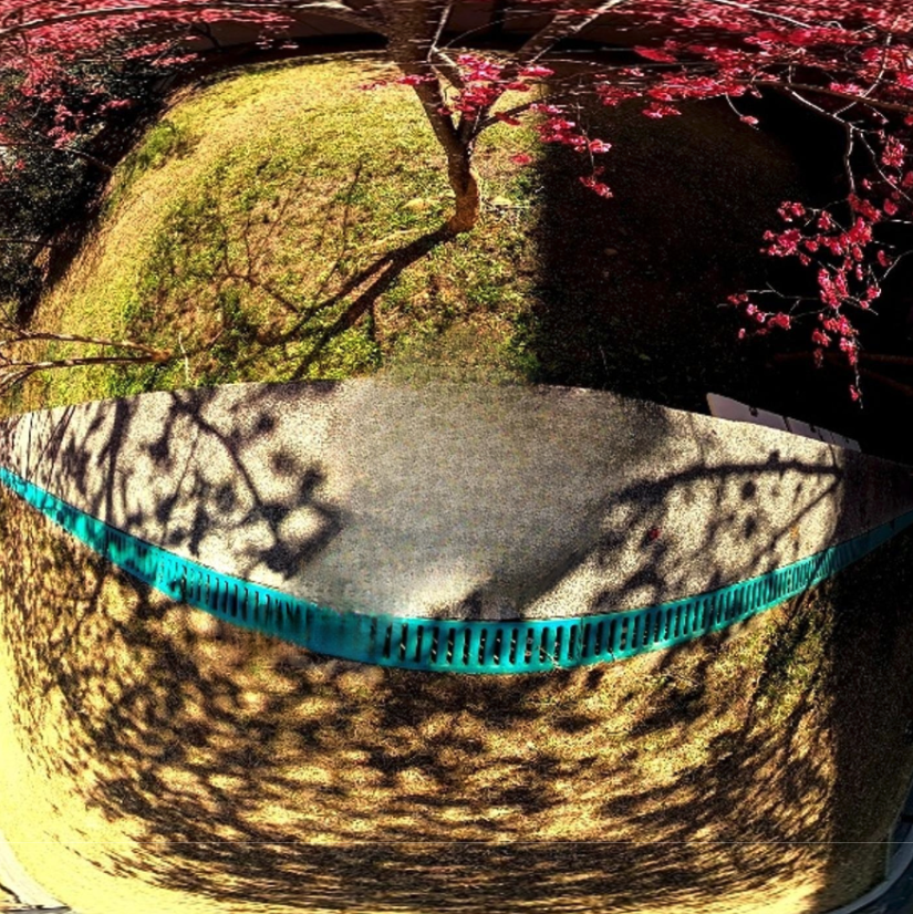
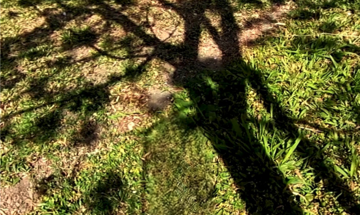
Stationary video Example #1: a 360° video taken by a hand-held camera. We want to mask out the red cameraman along with his shadow.


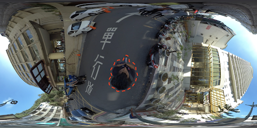
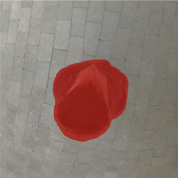
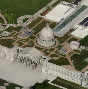
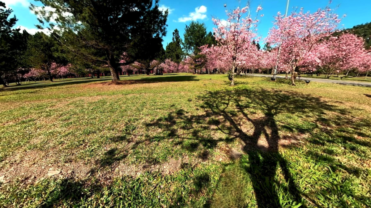
Stationary video example #2: a 360° video taken by a camera mounted on a tripod, we want to mask out the tripod in the center.


Although it can be difficult to classify a video as stationary or dynamic at times, (e.g. videos in which the cameraman alternately walks and stands), we still find it very helpful to do so, since these two types of video have very different natures and thus require different approaches to remove the cameraman.


Why Do We Treat Stationary Videos and Dynamic Videos Differently?

The reason we have classified videos as dynamic and stationary is that previous cameraman removal algorithms [1] were unable to provide realistic content for the masked area when the camera is stationary.  By analyzing the properties of stationary videos, we developed a separate CMR algorithm tailored to target their special settings.

We discuss in the following sections two challenges induced by stationary videos that must be taken into account when developing high-quality CMR algorithms.

Challenge 1: “Content Borrowing” Strategy Fails on Stationary Videos


What is “Content Borrowing” ? How does Previous CMR Method Work?

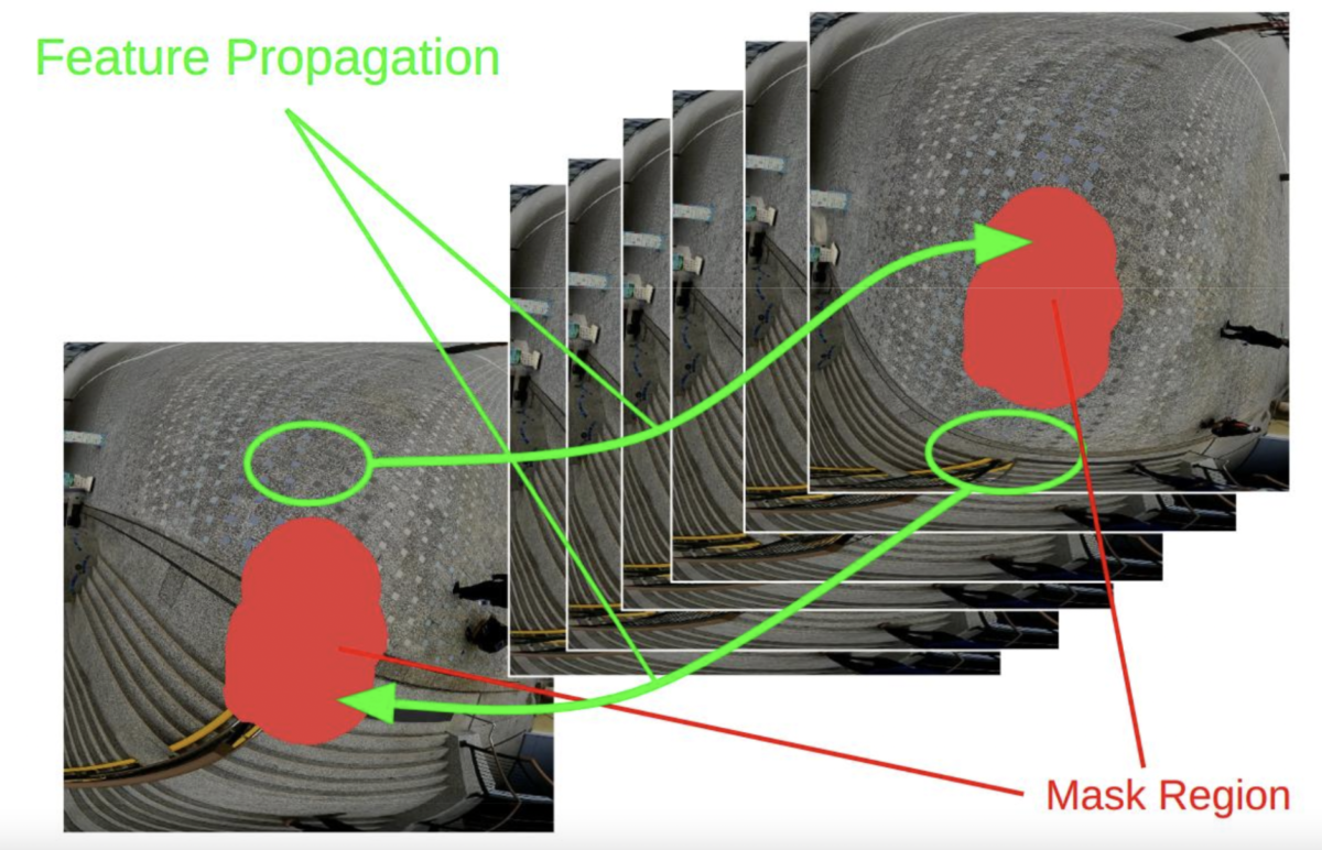
As shown in the diagram, flow-guided video painting methods (e.g. FGVC[2] , which is used by our previous CMR method[1] ) draw frames sequentially from bottom-left to top-right. To generate the content of the masked region (red region), we detect the relative movement of each pixel between neighboring frames, and borrow (green arrows) the content of the currently masked region from neighboring frames that might expose the target region as the camera moves.


In the dynamic video, where the cameraman is walking, masked regions almost certainly become visible in future frames as the masked content changes along the video. That is why “content borrowing” works well on dynamic videos.


CMR result on dynamic videos with “feature borrowing” strategy (generated by previous CMR method based on FGVC)


Content Borrowing on Stationary Videos

When CMR is used on stationary videos, if the mask is also stationary (which is often the case since the cameraman tends to maintain the same relative position to the camera throughout the entire video), then the content of the masked region might not be exposed for the duration of the video. Thus, in order to fill in the masked area, our stationary CMR algorithm must “hallucinate” or “create” realistic new content on its own.


Challenge 2: Human Eyes are More Sensitive to Flickering and Moving Artifacts in the Stationary Scene

When designing CMR algorithms for stationary videos, we encountered another challenge because human eyes are more sensitive in stationary videos than in dynamic videos. Specifically, any flickering or distortion in a video without camera movement will draw the viewer’s attention and disturb their viewing experience.

  • As we run the previous CMR method on stationary videos, we can observe obvious artifacts associated with warping and flow estimation errors.
  • In spite of the fact that we use the same mask generation method for both stationary and dynamic videos, the tiny disturbance in the mask boundary is considered an artifact in stationary videos, while it is silently ignored by viewers in dynamic videos.


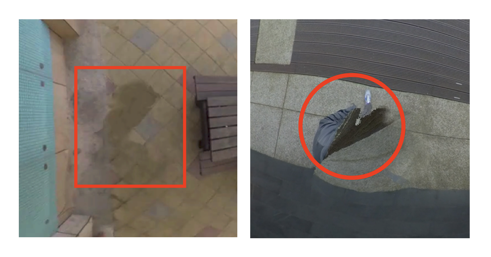
The result of the previous method (based on FGVC[2]) on stationary videos: Note the texture mismatch around the mask boundary due to warping, and the content generation failure in the bottom left corner.


The human eye can detect even tiny inconsistencies in the mask boundary when watching stationary videos. Although the mask boundary in the inpainted result appears natural in each individual frame, there is still disturbing flickering when the boundary changes between frames. In a dynamic video, this artifact is hardly noticeable.

According to the properties of stationary video outlined above, we propose three possible solutions, whose concept and experimental results are presented in the next section.


Three Stationary CMR Solutions

Our three different solutions share the same preprocessing steps:

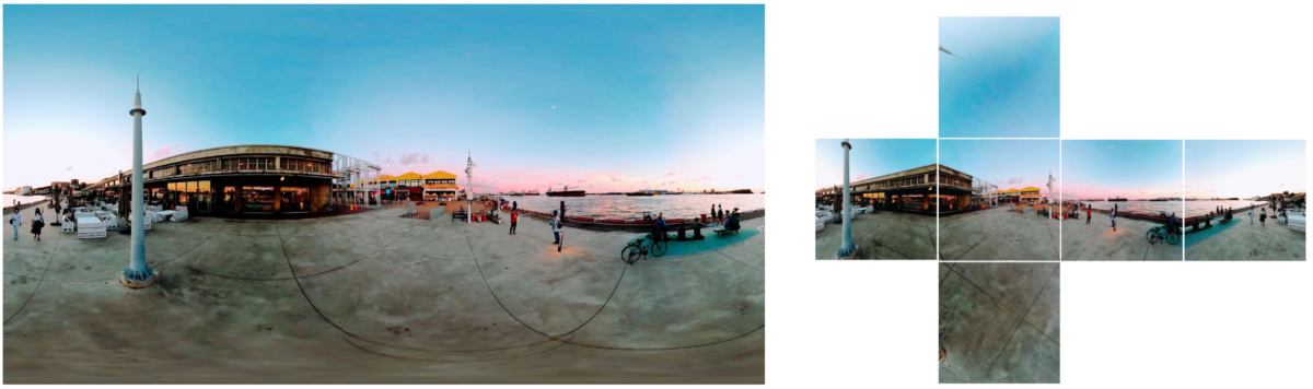
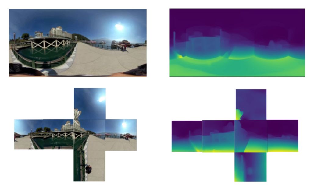
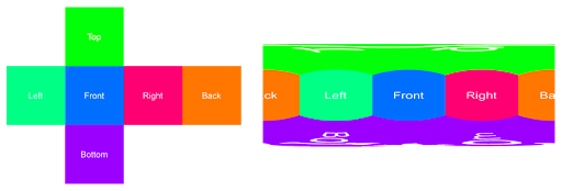
  1. We first convert 360° video into an equirectangular format
  2. Then rotate the viewing direction so that the mask is close to the center region.
  3. Finally, a square-shaped region containing the mask and its surrounding area is cropped and resized to a suitable input resolution for each solution. 

In addition, after the CMR has been completed, we upsample the result using the ESRGAN super-resolution model [3] before pasting it onto the original 360° video.

All three solutions utilize image inpainting models as a common component. It is preferred to use image inpainting models because they are capable of hallucinating realistic content more effectively than video inpainting models, which rely heavily on the “content borrowing” strategy. Also, video inpainting models are trained using only video datasets, which contain less diverse content than image datasets. The following experiments are conducted based on the LaMa [4] model for image inpainting.


In a simplified perspective, our three different solutions are essentially three different ways to extend the result of the LaMa [4] image inpainting model (which works on a single image instead of video) into a full sequence of video frames in a temporally consistent and visually reasonable manner.

Solution #1: Video Inpainting + Guidance

Our solution #1 aims to make video inpainting methods (which are normally trained on dynamic videos) applicable to stationary videos by modifying them. After testing various video inpainting methods, we selected E2FGVI [5] for its robustness and high-quality output.


We can divide our experiment on video inpainting into four stages.

1.Naive Method

Firstly, if we run a video inpainting model directly on the stationary input video, we will obtain poor inpainting results as shown below. The model is unable to generate realistic content because it is trained exclusively on dynamic video, and therefore heavily relies on the “content borrowing” strategy previously described.


2. Add Image Inpainting Guidance

In order to leverage the power of the video inpainting model, we design a new usage for our video inpainting model that makes the “content borrowing” strategy applicable to stationary videos. In particular, we insert the image inpainting result in the first frame of the input sequence and remove the mask corresponding to it, so that the video inpainting model can propagate the image in painted content from the first guiding frame to the later frames in a temporally consistent manner.

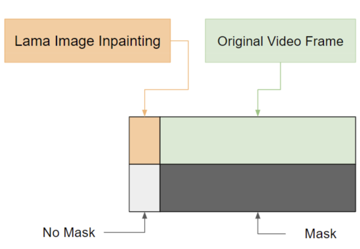
Modified input to video inpainting model: we insert the image inpainting result at the beginning of the input sequence to provide guidance to the video inpainting model.


After inserting guiding frames, we can see that the result is much more realistic.


There is, however, an inconsistent and strange frame in the middle of the above video. There is a complex reason for this:

  1. Due to the limitations of E2FGVI [5], we can only process at most 100 frames per run with VRAM on a single NVIDIA RTX3090 GPU. (We have observed similar memory constraints in our experiments using other deep-learning-based video inpainting implementations.)
  2. Due to this, we must divide our input video into multiple slices and process each slice separately. In this case, each slice contains 100 frames.
  3. Since each run is independent of the other, we must insert image inpainting guidance on each slice.
  4. There is a discrepancy between the resolution and texture quality of the inserted guiding slice generated by LaMa [4] and the video inpainted slice generated by E2FGVI [5], contributing to flickering artifacts in the transition between pairs of slices.

We will deal with this artifact in the next stage.

3. Softly Chaining the Video Slices together

In order to resolve the inconsistent transitions between consecutive slices, as described at the end of the previous stage, we attempted to use the last frame of the previous slide as the guiding frame for the next slice. Below is the result. This method suffers from accumulated content degeneration. After several iterations, the inpainted region becomes blurry.


Based on these results, it appears that the guiding information in the inpainted region decays when propagated across slice boundaries. Therefore, we propose a “soft chaining” method that mitigates the flickering artifact while preserving the guiding frames in each slice.


In particular, we modify the chaining mechanism so that each pair of neighboring slices has an overlap period during which the video is smoothly cross-faded from the previous slice to the next slice. Thus, we can still insert the guiding frame, but the guiding frame will be obscured by the overlapping crossfade. As a result, the flickering artifact is eliminated, and we are able to transit between slices smoothly.


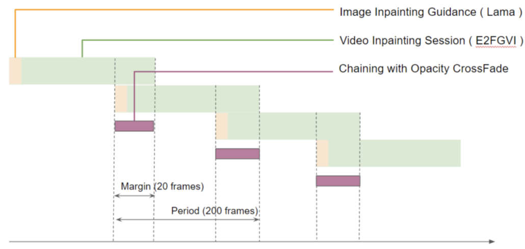
The soft chaining method for having smooth transitions between slices.


The result of Soft Chaining: We can see that the gap between each slice is less obvious.

4. Temporal Filtering 

Lastly, we eliminate vibration artifacts in our model by using a temporal filtering technique. The details of temporal filtering will be discussed in solution #3. Below is the final result (see Appendix 1 for 360° results):


One of the main artifacts of Solution #1 is the crossfade transition between neighboring slices. Although the transition is visually smooth, it is still disturbing in the stationary video. Another artifact is the unnatural blurry blob in the center of a large mask. It is likely that the artifact is caused by the limitations of the architecture of E2FGVI_HQ, which produces blurry artifacts in regions far from the inpainted boundary. These artifacts will be considered in the comparison section below.


Solution #2: Image Inpainting + Poisson Blending

In solution #2, we attempted to “copy” and “paste” the inpainted region of the first frame to other frames within the scene by using Poisson blending.

The Poisson Blending [6] technique is a technique that allows the texture of one image to be propagated onto another while preserving visual smoothness at the boundary of the inpainted area. Here is an example of the seamless cloning effect shown in the original paper [6]:

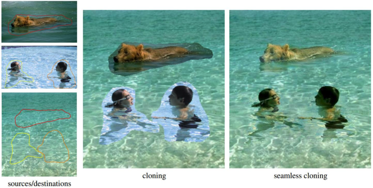
As a result of the properties of Poisson blending, when we clone the image inpainting result of LaMa [4] to the rest of the video frames, the copied region automatically adjusts its lighting in accordance with the surrounding color on the target frame.


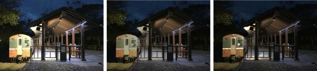
Poisson Blending Good Result #1: It works well on a time-lapse sunrise video since Poisson blending ensures a smooth color transition within the mask area.


Poisson Blending Good Result #2: In comparison with the other two methods, Poisson blending offers a very stable inpainting region across frames.


Poisson blending, however, is only applicable to tripod videos, not to handheld stationary videos, since it assumes that the inpainted content won’t move throughout the video. We can see in the example below that the inpainted texture is not moving with the surrounding video content, resulting in an unnatural visual effect.


Poisson Blending on Handheld Video (Bad Result): The inpainted texture does not move with the surrounding video content, causing unnatural visual effects.


Poisson Blending on Tripod Drift: A tripod video may also contain tiny camera pose movements that accumulate over time, resulting in the inpainted content drifting away from the surrounding area of the frame.


Solution #3: Image Inpainting + Temporal Filtering

In solution #3, we take a different strategy. Instead of running image inpainting on only the first frame of the input sequence, we run it on all frames. The following result is obtained.


 This result is very noisy since LaMa [4] generates content with a temporally inconsistent texture. In order to mitigate the noisy visual artifact, we apply a low-pass temporal filter to the inpainted result. A temporal filter averages the values pixel-by-pixel across a temporal sliding window so that consistent content is extracted and the high-frequency noise is averaged out. Below is the result after filtering (for 360° video results, please refer to Appendix 2):


At first glance, the result appears stable, but if we zoom in and observe closely, we will see that the color of every pixel gradually changes, resulting in a wavy texture. 


As shown below, we also observe white-and-black spots in the results, which we refer to as the “salt and pepper artifact”. This artifact is the most disturbing artifact of Solution #3 and will be discussed later.


Solution #3 Result Zoomed In: We can see salt and pepper Artifacts and tiny flickering caused by super-resolution models.

As we have described all three solutions, the next step will be to compare them and select the one that best meets our requirements.

Comparing and Choosing from Experimental Solutions

The results of previous experiments demonstrated that each solution has its own advantages and weaknesses, and there was no absolute winner which outperformed every competitor in all circumstances.

Quality Comparison

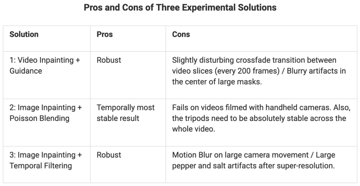
Based on the results of the experiment, we estimate for each solution its potential quality of achieving our project goal in order to determine one final choice for further refinement. The experimental results of each solution were converted into 360° videos and then evaluated by our photographers and quality control colleagues. The following table summarizes the pros and cons of each solution.

Speed Comparison

We also tried to take into account the running speed of each solution when choosing the solution. However, at the experiment stage, it is difficult to determine the optimal speed of each solution since we expect to see a large speed up if we implement the entire pipeline on the GPU. During the experimental pipeline, intermediate results are saved and loaded to disk, and image frames are unnecessarily transferred between GPU and CPU. Due to the similar speed of each algorithm, we did not consider the computation cost of each solution when making our decision.

Conclusion 

Based on the qualitative comparison and feedback from the photographer and the quality control department, the following decisions were made.

  • Solution #2 was the first one to be eliminated from the list due to its low robustness (it only works with perfectly stable tripod videos).
  • Based on the feedback voting, solution #1 and solution #3 performed equally well, so we compared their potential for further refinement:
    • It is difficult to fix blurry artifacts in the mask center of Solution #1 due to the architecture of the video inpainting model.
    • In Solution #1, the crossfade transition caused by memory constraints is also difficult to resolve.
    • By adjusting the resizing rules of our pipeline, we may be able to resolve the pepper and salt artifact (which is the most complained-about downside of Solution #3).

Therefore, we chose solution #3 since it is more likely to be improved through further finetuning.


Fine-tuning for Solution #3 (Image Inpainting + Temporal Filtering)

The Solution #3 algorithm has been further optimized in three different aspects: 

  1. Identify the origin of salt and pepper artifacts and remove them
  2. Remove the flickering mask boundary
  3. Speed up.

Identify the Origin of Salt and Pepper Artifacts

Here is the diagram of the solution #3 CMR pipeline, in which we search for the cause of the artifact.


It turns out that the artifact is caused by the resizing of the image before inpainting. During the resizing stage, we resize the cropped image from 2400×2400 to 600×600. However, at resolution 600×600, the image suffers severe aliasing effects, which are preserved by LaMa in the inpainted region (as shown below), resulting in black and white noise pixels. In the following stage, the super-resolution model amplifies the noise pixels further.

Output of the LaMa image inpainting model: The aliasing effect in the context region is replicated by LaMa in the inpainted region.

Inpainted Region after super-resolution and overwriting mask area: It can be seen that the black and white noise pixels in the inpainted area have been further amplified by the super-resolution model. The context area that is not overwritten remains unchanged.


Removing Salt and Pepper Artifacts

The idea is to reduce the scaling factor of the resize process so that more detailed information can be preserved and there will be less aliasing. To achieve this, we made two modifications: 1. Increase the LaMa input dimension and 2. Track and crop smaller regions around the mask.

Increase LaMa Input Dimension

We tested different input resolutions and found that LaMa [4] can handle input sizes greater than 600×600. However, we are unable to feed the original 2400×2400 image into LaMa. When the input image is too large, we receive an unnatural repetitive texture in the inpainting area. Experimentally, we find that the optimal operating resolution and content quality trade-off lies around 1000×1000, so we change the resizing dimension before LaMa to 1000×1000.

Input size=600×600:
many salt and pepper artifacts due to extreme resizing scale.

Input size=1000×1000:
good inpainting result

Input size=1400×1400:
we can see unnatural repetitive texture inside the inpainted area.


Track and Crop Smaller Region Around the Mask 

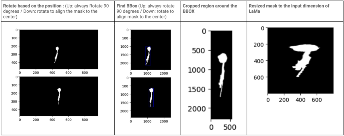
Another modification that improves the inpainting quality is to crop a smaller area of the equirectangular video. By using smaller cropped images, we can use smaller resize scales in order to shrink our input to 1000×1000, preserving more detail in the final result. The cropping area should include both the masked region as well as the surrounding regions of the mask from which LaMa [4] can generate plausible inpainting content. Our cropping mechanism is therefore modified so that it tracks both the mask’s position and shape. Specifically, instead of always cropping the center 2400×2400 region of the rotated equirectangular frame, we rotate the mask region to the center of the equirectangular frame and crop the bounding rectangle around the mask with a margin of 0.5x the bounding rectangle’s width and height. Below is an illustration of the mask tracking process.


Rotate and crop the equirectangular frame based on the position and shape of the mask: By using this method, the cropped image would be smaller, thus reducing the resizing scale and improving the quality of the image.

Remove ESRGAN Super-Resolution Model

With the above two modifications, we discovered that the scale factor was drastically reduced, so that the super-resolution module was no longer required. Therefore, we replaced the ESRGAN super-resolution model with normal image resizing, thereby further eliminating salt and pepper artifacts.

Removing Flickering Mask Boundary

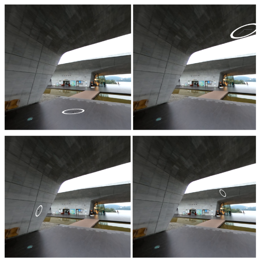
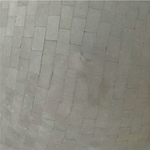
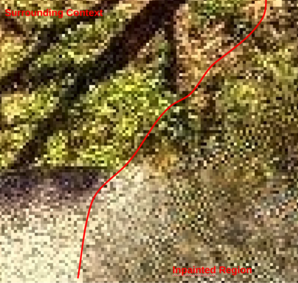
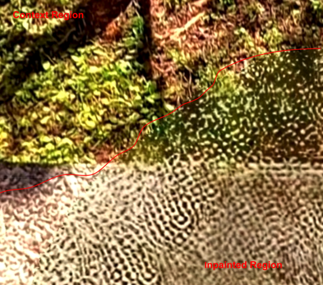
Can you find the boundary of the inpainted mask in the picture below?

It should be difficult to detect the inpainted mask even when zooming in.

Nevertheless, if the mask boundary is inconsistent across frames, we can observe a flickering effect that reveals the existence of an inpainting mask.


In order to remove the artifacts, we apply temporal filtering on the binary mask before feeding it to the CMR pipeline.Furthermore, we continuously blur the mask when we paste the inpainted region back into the 360° video.

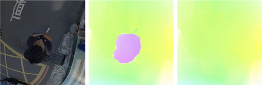
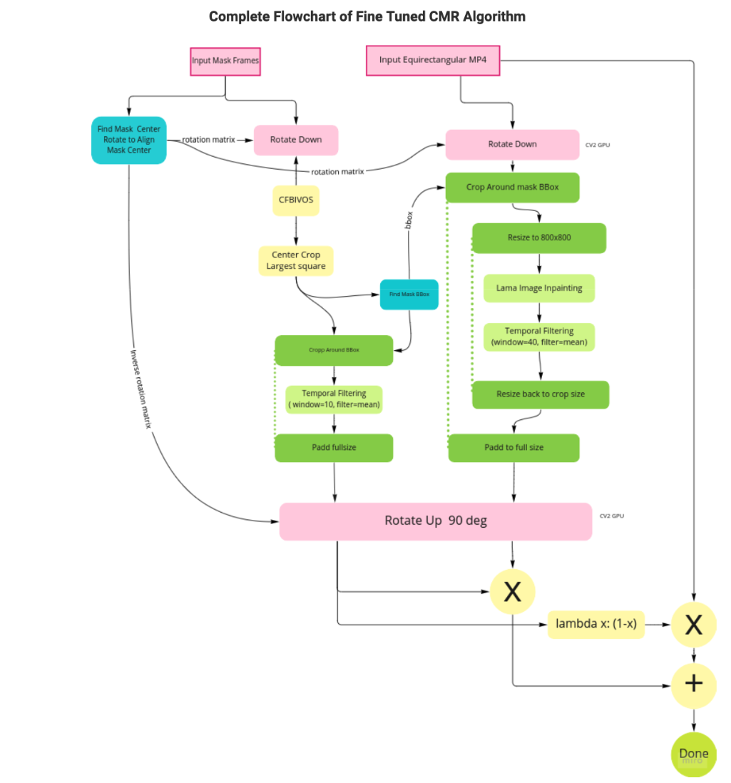
Please refer to the following flow chart for a detailed explanation of our fine-tuned CMR algorithm based on Solution #3. We can see that 

  1. In the blue parts, we rotate the input mask based on the position of the mask, and then crop the mask based on the BBox around the rotated mask.
  2. We apply temporal filtering to both the mask output of CFBVIO [7] and the frame output of LaMa.

Speeding Up 

As part of the fine tuning process, we also made the following modifications in order to speed up the algorithm:

  1. Preprocessing of LaMa models is now performed on GPUs rather than CPUs
  2. All the processes in the CMR are chained together, and all the steps are executed on a single GPU (RTX3090).
  3. The CMR algorithm and the video mask generation algorithm [7] are chained together with a queue of generated mask frames provided by a Python generator, so that the two stages can run simultaneously on a single GPU.

Following these fine-tunings, the final CMR and mask generation model [7] run at 4.5 frames per second for 5.6k 360° videos.

Conclusion 

We have presented here the final results of our fine-tuned stationary CMR algorithm in 360° format (see Appendix 3 for additional results, and Appendix 2 for the results before fine-tuning). As can be seen, the fine tuned method successfully removed the pepper and salt artifacts, as well as stabilizing the mask boundary.

Visually, the inpainted area is reasonable, as well as temporally smooth. Compared to previous methods, this algorithm successfully achieves the goal of CMR under the constraints of stationary video, and greatly enhances the viewing experience.

The following three points summarize this blog article:

  1. Our study compares the properties of stationary and dynamic videos, and analyzes the challenges of developing CMR algorithms from stationary videos.
  2. On the basis of these observations, we propose three different solutions for CMR and compare their strengths and weaknesses.
  3. Solution #3 is selected as our final algorithm and its performance is further fine-tuned in terms of quality and speed.

In the case of stationary video, our algorithm is capable of handling both tripod and handheld video and it achieves much better results than the previous method while being much faster.

References 

[1] AILABS.TW, “The Magic to Disappear Cameraman: Removing Object from 8K 360° Videos Taiwan AILabs.” https://ailabs.tw/smart-city/the-magic-to-disappear-cameraman-removing-object-from-8k-360-videos/ (accessed Jun. 13, 2022).

[2] C. Gao, A. Saraf, J.-B. Huang, and J. Kopf, “Flow-edge Guided Video Completion,” arXiv, arXiv:2009.01835, Sep. 2020. doi: 10.48550/arXiv.2009.01835.

[3] X. Wang et al., “ESRGAN: Enhanced Super-Resolution Generative Adversarial Networks.” arXiv, Sep. 17, 2018. doi: 10.48550/arXiv.1809.00219.

[4] R. Suvorov et al., “Resolution-robust Large Mask Inpainting with Fourier Convolutions.” arXiv, Nov. 10, 2021. doi: 10.48550/arXiv.2109.07161.

[5] Z. Li, C.-Z. Lu, J. Qin, C.-L. Guo, and M.-M. Cheng, “Towards An End-to-End Framework for Flow-Guided Video Inpainting,” arXiv, arXiv:2204.02663, Apr. 2022. doi: 10.48550/arXiv.2204.02663.

[6] P. Pérez, M. Gangnet, and A. Blake, “Poisson image editing,” in ACM SIGGRAPH 2003 Papers, New York, NY, USA, Jul. 2003, pp. 313–318. doi: 10.1145/1201775.882269.

[7] Z. Yang, Y. Wei, and Y. Yang, “Collaborative Video Object Segmentation by Multi-Scale Foreground-Background Integration,” arXiv, arXiv:2010.06349, May 2021. doi: 10.48550/arXiv.2010.06349.


Appendix 1: 360° Video Results of Solution #1


Appendix 2: 360° Video Results of Solution #3 Before Fine Tuning


Appendix 3: 360° Video Results of Solution #3 After Fine Tuning


Hovering Around a Large Scene with Neural Radiance Field

Video 1: Hovering around A LI Mountain with neural radiance field


Introduction

Neural Radiance Field (NeRF) [1] has been a popular topic in computer vision since 2020. By modeling the volumetric scene function with a neural network, NeRF achieves state-of-the-art results for novel view synthesis.


While NeRF-related methods are popular in academia, they have not been widely implemented on products to provide user experiences. This article aims to demonstrate how Neural Radiance Field can be used to create an immersive experience for users hovering around a large attraction sight.


Background

Neural Radiance Field [1] is an avant-garde way of predicting novel views from existing images. While traditional 3D reconstruction methods estimate a 3D representation of the scene using meshes or grids, NeRF overfits a neural network to a single scene and determines how every 3D point looks from a novel viewpoint in that scene. Through ray tracing and L2 image construction loss, the model tries to predict the color and volume density of every point in the scene from several training images of the scene with known camera poses.


Since the publication of NeRF, there have been several follow-up studies. By rendering conical frustums instead of rays, Mip-NeRF [2] eliminates aliasing without supersampling. Through modeling the far-scene differently from the near-scene, Mip-NeRF 360 [3] and NeRF++ [4] achieve better visual results in the “background scenes”. Via storing features in local scenes, Instant-NGP [5] and Point-NeRF [6] allow the models to encode large scenes and converge quickly during training. By combining multiple neural radiance fields, Block-NeRF [7] allows the models to encode even larger scenes such as an entire neighborhood of San Francisco.


Improving NeRF for Encoding Large Scenes 

The first step towards encoding a large attraction sight in a neural radiance field is choosing a model structure suitable for our use case. Despite NeRF’s great performance on small 360-degree scenes, encoding large complex scenes in NeRF is not feasible due to its simple MLP encoding method. Also, Mip-NeRF 360 and NeRF++ do not allow users to hover too far around the scene since the far scene is encoded differently than the near scene. Finally, although Block-NeRF is capable of modeling large scenes well, it also takes a considerable amount of time and computing power to train. On the other hand, by storing trainable local features in hash tables and treating the near and far parts of a scene in the same way, Instant-NeRF can create a large neural radiance field where users can hover freely. As a result, in this project, we will exploit Instant-NGP’s method of storing local features in the scene. Also, we utilize COLMAP [8] to compute camera poses for input images. However, to encode an attraction site and let users hover around, we still need to get enough viewpoints in training data and remove dynamic objects.


Getting Enough Viewpoints in Training Data

Video2: Instant-NeRF does not work well on extrapolating colors from unseen angles


Video3: Our method improves image quality from a variety of viewpoints


Unlike traditional 3D reconstruction methods, neural radiance fields allow objects to appear in different colors from different angles. However, Instant-NeRF does not work well on extrapolating colors from unseen angles (see video 2). Thus, to encode a scene in Instant-NeRF, we need a filming strategy that can allow our model to see from a variety of angles. 

Traditionally, Instant-NeRF assumes all training images point to a common focus. However, we found that this kind of filming strategy works best for encoding objects, but not large scenes. When filming a large scene, we may not always have a visible common focus across images. Also, we may need more flexible techniques for encoding large complex scenes since they often contain more complex objects and occluded areas.

To get enough different angles, we develope a new filming method for filming perspective input images. To elaborate, we both circle the scene to film 360° inward videos and films from different heights such that the model has enough information to predict color from different angles. We then sample the video 2 frames per second to ensure COLMAP gets enough common features to compute camera poses. 

In addition, our system supports the input of 360° videos. Traditionally, Instant-NeRF and COLMAP support only perspective input data. To the best of our knowledge, we are the first to use 360° videos in training Instant-NeRF. In general, one won’t consider forward-walking 360° videos suitable for Instant-NeRF training since they lack common focus even if there is no occluded space. However, we found that a 360° video can lead to great results for encoding a large scene since it satisfies two conditions: COLMAP has enough common features to match among frames, and Instant-NeRF has a wide variety of training data for interpolating the color for every point in the space. When utilizing 360° videos from Taiwan Traveler, we first convert the sampled panoramic view into perspective images. A common way to do this is to project a spherical 360° image onto a six-face cube map. We found that COLMAP can accurately estimate the camera pose of cube map images. As a result, we can convert equirectangular images to the format that Instant-NeRF supports and produce high-quality results. Furthermore, we provide the option to dump the vertical images in outdoor scenes since they usually contain little information about the scene and could potentially spoil the model with misleading camera poses. With 360° videos, we found that we can get better results with easier filming techniques.


Picture 1: Converting a 360° equirectangular image (left) to a cube map (right). Vertical images in the cube map (the up and down ones) usually contain less information about the scene


Picture 2: Perspective (left) and 360° (right) filming methods, with the green pyramids being camera positions

Dynamic Object Removal

When encoding a popular site, chances are there will be many people or cars moving around in the scene. Moving objects could be a challenge to Instant-NeRF and COLMAP because both assume input data to be static.

To tackle this issue, we utilized a pre-trained image segmentation model, DeeplabV3 [9], to mask popular moving objects such as people and cars. Following our previous work [10], we can also obtain masks of cameramen. Then, we ignore those masked objects both when extracting features for computing camera poses and ray tracing during training Instant-NeRF.

Picture 3: Masking popular dynamic objects with DeeplabV3

Applications

With the ability to edit camera paths after filming videos, directors can now create many novel videos with different camera paths based on only one set of training images. We integrate Potree[11], an open-source WebGL point cloud viewer, and Instant-NeRF to develop a studio that allows creators to edit desired camera movements. To elaborate, after encoding the whole tourist site, Potree visualizes the sparse points output by COLMAP so that creators can assign camera paths and produce immersive hovering-around videos using the studio.

Video6, 7: Assign the camera path in Potree (up) and then render a video with novel views (down)


To implement Instant-NeRF for a real-time, interactive experience, we deploy Instant-NeRF on a local device with high GPU memory. Moreover, we can allow users to fly around scenes immersively by combining human pose estimation.


Conclusion

In this article, we demonstrate how to encode large scenes in neural radiance fields and let users edit camera paths afterward or fly around the field interactively. We achieve it by developing a pipeline that can transfer both 360-degree and perspective videos into a new video with novel paths. We also provide guidelines on filming techniques for encoding a large scene and tackle common issues when implementing Neural Radiance Field in the field such as path assignment and dynamic object removal. 

Video8~11: Hovering around famous tourist attractions in Taiwan with Instant-NeRF. From top to bottom, they are results of Kaohsiung Pier-2 Art Center, Xiangshan Visitor Center, Taipei Main Station, and Sun Moon Lake


Reference

  1. Ben Mildenhall and Pratul P. Srinivasan and Matthew Tancik and Jonathan T. Barron and Ravi Ramamoorthi and Ren Ng. (2020). NeRF: Representing Scenes as Neural Radiance Fields for View Synthesis. ECCV 2020
  2. Jonathan T. Barron, Ben Mildenhall, Matthew Tancik, Peter Hedman, Ricardo Martin-Brualla, and Pratul P. Srinivasan. (2021). Mip-NeRF: A Multiscale Representation for Anti-Aliasing Neural Radiance Fields. CVPR 2021
  3. Jonathan T. Barron and Ben Mildenhall and Dor Verbin and Pratul P. Srinivasan and Peter Hedman (2022). Mip-NeRF 360: Unbounded Anti-Aliased Neural Radiance Fields. CVPR 2022
  4. Kai Zhang, Gernot Riegler, Noah Snavely, Vladlen Koltun (2021). NeRF ++: Analyzing and Improving Neural Radiance Fields.  arXiv:2010.07492
  5. Thomas Muller, Alex Evans, Christoph Schied, and Alexander Keller (2022). Instant Neural Graphics Primitives with a Multiresolution Hash Encoding. ACM Trans. Graph. July 2022
  6. Qiangeng Xu, Zexiang Xu, Julien Philip, Sai Bi, Zhixin Shu, Kalyan Sunkavalli, Ulrich Neumann (2022). Point-NeRF: Point-based Neural Radiance Fields. CVPR 2022
  7. Matthew Tancik, Vincent Casser, Xinchen Yan, Sabeek Pradhan, Ben Mildenhall, Pratul P. Srinivasan, Jonathan T. Barron, Henrik Kretzschmar (2022). Block-NeRF: Scalable Large Scene Neural View Synthesis. CVPR 2022
  8. Schonberger, Johannes Lutz and Frahm, Jan-Michael. (2016) Structure-from-Motion Revisited. CVPR 2016
  9. Liang-Chieh Chen and Yukun Zhu and George Papandreou and Florian Schroff and Hartwig Adam. (2018) Encoder-Decoder with Atrous Separable Convolution for Semantic Image Segmentation. ECCV 2018
  10. Taiwan AI Labs. The Magic to Disappear Cameraman: Removing Object from 8K 360° Videos (2021)
  11. Potree, WebGL point cloud viewer for large datasets, at potree.org

It is Enough to Take Only One Image: Re-exposure Images by Reconstructing Radiance Maps

Fig. 1 (Left) original image (Middle) result image of adjusting the brightness directly (Right) result image of adjusting the exposure on our reconstructed radiance map.

Nowadays, more and more people like to take pictures with smartphones and post on social media to share beautiful photos with their friends. Usually, they do some image editing before they post, such as applying filters, adjusting color warmth, saturation or contrast. However, there is one thing they can never change unless they go back to the place where they took the photo and shoot again, i.e., exposure, a parameter that is fixed forever after you click the shutter button. Although it is possible to simulate exposure change effects by adjusting the picture’s brightness, like the middle image of Fig.1, existing tools do not allow us to recover the details of an over-exposed or under-exposed region due to the limitations of the camera sensor.  We propose to solve this issue by reconstructing the radiance map for the image and using GANs to predict the ill-exposed regions. See the right image of Fig.1 as an example. We can recover the missing details on the train (see Fig. 2 to get a closer look), making the result more realistic. With our technique, users can adjust the exposure parameter to have the image they want without going back to the place and taking it again. We will focus on building the model to reconstruct the radiance map in the following and provide more results.


Background

We first explain the jargon to provide background knowledge to the readers. If you are  familiar with them, feel free to skip this section.

  • Radiance map: a map that records the true luminance value of the scene. The channel value of a pixel is usually represented by a real number with a large range. We also name it HDR image in this article at times. 
  • HDR image: abbreviation of High Dynamic Range image, identical to the term radiance map in the article. 
  • LDR image:  abbreviation of Low Dynamic Range image. It is the conventional image, where the channel value of a pixel is represented by an 8-bit number, ranging from 0 to 255. LDR images can be generated by tone mapping from the HDR image and displayed on normal screens. 
  • Tone mapping: the process of mapping an HDR (high dynamic range) image to an LDR (low dynamic range) image which can be displayed.

Fig. 2 A closer look of the difference between (Left) naive brightness adjustment and (Right) our result.

Our Method

In the camera, the sensor array records pixels’ values according to the scene radiance and the exposure setting. Due to the limited range of the sensor, excessive values are clipped. To better human perception, the values are nonlinearly mapped using the CRF (camera response function). Finally, the values are quantized and stored into an 8-bit number. The processes of clipping, nonlinear mapping, and quantization all lead to information loss. 

Inspired by [1], we reconstruct the HDR image by reversing the camera pipeline. Starting from an input LDR image, we inverse the CRF by simply applying a square-root mapping. At the next step, we let the model predict values of over-exposed regions, which are clipped by the camera to reconstruct the HDR image. Two key features differentiate our method from other HDR reconstruction methods [1,4,5,6]. The first one is the architecture; unlike Liu et al. [1], which uses an encoder-decoder network to predict values, we treat value prediction in the over-exposed region as an inpainting task in the linear space because GANs can generate better and more realistic results. The second one is that we predict relative luminance instead of absolute luminance. Our goal is to get correct brightness changes and details when applying different exposure parameters, so it is more important to get relatively correct values.

Also, predicting relative luminance is more manageable than predicting the absolute one. About the architecture, we use the U-Net with gated convolution [2] layers (Fig. 3). We also add skip connections, as our experiment shows that they offer clearer and more realistic results. For the discriminator (Fig. 4), we use SN-PatchGAN [2]. Instead of passing the predicted HDR image to the discriminator, we pass the LDR image as the input of the discriminator network. Our experiment shows that passing an image in the linear space as input will cause artifacts in the results. We tone-map an HDR image to an LDR image by directly clipping the value to [0-1] and applying a naive CRF to simulate digital cameras.  

Fig. 3 Our generator model.


Fig. 4 Our discriminator model (SN-PatchGAN in [2]).


Dataset

Data cleaning

We use the dataset provided by singleHDR [1]. However, we found that images of the dataset record relative luminance. Thus the same scene can have different value scales. The scale differences could confuse the model and get worse results. For addressing that issue, we perform data normalization before training to make most pixels (95% in our case) range within [0-1]. This way,all values are of a similar scale so that the model can predict more stably.

Data augmentation

For previous methods [4, 5, 6] that predict absolute luminance, the data augmentation process generates LDR images by applying different CRF curves to the same HDR image to create additional data pairs. They expect those LDR images to be reconstructed into the same HDR image, so they generate data pairs like [GT-HDR, LDR-ev+3], [GT_HDR, LDR-ev+0], [GT_HDR, LDR-ev-3]. For our method, which predicts relative luminance, our data augmentation process generates LDR images by applying different CRF curves to the same HDR image as others do. However, we will create data pairs [GT-HDR-ev+3, LDR-ev+3], [GT-HDR-ev0, LDR-ev0], [GT-HDR-ev-3, LDR-ev-3] (Fig. 5) because we predict relative luminance instead of absolute luminance.

Fig. 5 our data augmentation procedure ([0-1] means 95% of pixels have values in this range).

Loss function

Our loss function is composed of  the generator loss (mean-square loss in the log domain), discriminator loss, and perceptual loss. For the perceptual loss [3], it is worth mentioning that we experiment with which layer of features to use and whether to use the features before the activation layer or after. Different VGG net layers are well-known that encode different semantic features levels, so different tasks could use different layers for perceptual loss. Features before the activation layer and the ones after the layer have different data distributions and ranges, and both have been used in different researches. In our experiments, we get the best result by using the conv3_4 layer of VGG19 before the relu activation(Fig. 6).

Fig. 6 The perceptual Loss.


Results

We show two result videos using our method. Given the image shown at the left bottom, we adjust the exposure using our model. In Video1, our method recovers the ill-exposed region on the train (see Fig. 2 to get a closer look). In Video2, we can see the contour of streetlights more clearly as we darken the image.

Video1


Video2


360° Depth Estimation

360° videos provide an immersive environment for people to engage, and Taiwan Traveler is a smart online tourism platform that utilizes 360° panoramic views to realize virtual sightseeing experiences. To immerse users in the virtual world, we aim to exploit depth information to provide a sense of space, enabling tourists to better explore scenic attractions.


Introduction

Depth plays a pivotal role in helping users to perceive 3D space from 2D images. With the depth information, it is possible to provide users with more cues about the sense of 3D space via 2D perspective images. For example, a disparity map can be derived from the depth map, and it is possible to create stereo vision. Also, the surface normals can be inferred by the depth map for better shape understanding. By warping the cursor according to depth and surface normals, users can experience the scene geometry better through hovering over the images.

Depth estimation of perspective images is a well-studied task in computer vision, and deep learning has significantly improved its accuracy. Trained with large datasets containing ground-truth depth information, the estimation models learn to predict the 3D scene geometry by merely using 2D images. However, the depth estimation of 360° images is knotty. The estimation model’s ability is often limited to indoor environments because of the lack of datasets for outdoor scenes. In addition, the distortion on an equirectangular image makes the problem difficult to tackle with convolution neural networks. Thus, predicting accurate 360° depth maps from images is still a challenging task. 

In this project, given a single 360° image, we aim at estimating a 360° depth map, by which we can calculate the surface normals, allowing users to hover the scenes by moving mouses over images. To obtain depth maps that can achieve a satisfactory user experience, we utilize single-image depth estimation models designed for perspective images. For adapting these models to 360° images, our method blends depth information from different sampled perspective views to output a spatially consistent 360° depth map.


Existing Methods

Monocular depth estimation refers to the task that predicts scene depth from a single image. Recently, deep learning has been exploited to cope with this challenging task and has shown compelling results. Through a large amount of data, the neural network can learn to infer per-pixel depth value, thus constructing a complete depth map.

Currently, 360° depth estimation is more mature for indoor scenes than outdoor ones. There are a few reasons. First, it is more challenging to collect ground-truth depth for 360° images, and most existing models rely on synthetic data of indoor scenes. Second, current models often leverage structures and prior knowledge of indoor scenes. Our online intelligent tour system contains a large number of outdoor scenic attractions, along with indoor scenes. Thus, existing models for indoor settings do not apply to our applications. 


Our Method

In order to take advantage of the more mature monocular depth estimation for perspective images, our method first converts equirectangular images to perspective images. A common way is to project a spherical 360° image onto a six-face cubemap. Each face of the cubemap represents a part of the 360° image through projection. After converting a 360° image to several perspective images, a depth estimation model for perspective images, such as the one proposed by Ranftl et al. [1] can be applied. These models often extract features from these NFOV (normal-field-of-view) images and predict depth maps.

After obtaining the depth maps for NFOV images, the next step is to fuse those depth maps into a 360° depth map. For the fusion task, we have to deal with the following issues. 

1. Objects across different NFOV images

When projecting the 360° spherical image onto different tangent planes, some objects could be divided into parts. The segmented parts can not be recognized well by the estimation model and could be predicted with inaccurate depth. Besides, the same objects across different planes could lead to depth inconsistency when assembling the parts, leading to apparent seams.


2. Depth scale

In a perspective depth map, though the relative depth relationship between objects is roughly correct, the depth gradient may be drastically large, e.g., a decoration on a wall or a surfboard on the water. The distinct color and texture between nearby objects would cause dramatically different depth values even if they are almost on the same plane.

Their depth scales could be different between multiple perspective depth maps, making it difficult to fuse them to a 360° depth map. Though we can adjust their depth scales to match neighboring images globally by overlapping areas, it’s challenging to adjust objects’ depth values locally. In addition, a depth map is adjacent to multiple depth maps. Thus, we need to solve for globally optimal scaling factors.


3. Wrong estimation of vertical faces

Most of the training data for the depth estimation model are captured from normal viewing angles. The datasets lack images looking towards the top (e.g., sky and ceiling) or bottom (e.g., ground and floor) of the scenes. Thus, the learned models often cannot learn to predict the accurate depth maps for those views. Usually, the surrounding area of a horizontal perspective image is closer to the camera, while the center area is often deeper than other regions. In contrast, the center area of top/bottom views is often closer to the camera, and other regions are farther away. Thus, depth estimation of the top/bottom views is often less accurate as the wrong prior is used.


Figure 1: top-left: 360° image, bottom-left: cubemap images, bottom-right: cubemap depth maps, top-right: fused 360° depth map with seams.


Due to the aforementioned issues, a 360° depth map often suffers from apparent seams along the boundaries of depth maps after fusion. Our method first converts 360° images to cubemaps with a FOV (field-of-view) larger than 90 degrees. It guarantees the overlaps between adjacent faces. After that, the estimation model predicts the depth map for each image. We then project each perspective depth map to a spherical surface and apply equirectangular projection for manipulating them on a two-dimensional plane. To avoid dramatic change between depth maps, we adjust their values according to the overlapping area. Then we apply Poisson Blending [2] to compose them in the gradient domain. The depth gradients guide the values around the boundaries and propagate inside, retaining the relative depth and eliminating seams. Therefore, the depth values smoothly change across depth maps.

Additionally, we utilize different strategies to divide a 360° image into several perspective images. Apart from the standard cubemap projection, our method utilizes two approaches to divide images and combine perspective depth maps. 

The first approach is to use a polyhedron to approximate a spherical image. When projecting a 360° image to a tangent plane, the peripheral regions are distorted, affecting the depth estimation, especially when FOV is large. By projecting the spherical surface to multiple faces (more than 20 faces), we better approximate a sphere with a polyhedron to obtain less distorted features. Nevertheless, adopting appropriate criteria to select and blend those depth maps is crucial. When having more depth maps to blend, adjusting their depth scales becomes difficult. Also, seamlessly blending images creates gradual depth change along the boundary, acting like a smoothing operation. With more blending iterations for the depth maps, smoothing all the boundaries between them generates blurring artifacts. Choosing the proper part of depth maps and designing the process to fuse them is essential.

The second approach is opposite to the previous one, using fewer depth maps to blend. As mentioned earlier, the estimation model cannot tackle the vertical faces on the top and bottom. Therefore, even if the boundary between vertical and horizontal faces is smooth, the predicted vertical depth maps’ gradient still contradicts our perception of real-world space. As such, we only predict the depth maps of horizontal perspective images and exploit them to generate a 360° depth map. We expand their FOV to obtain more information and increase overlapping. Besides, the vertical perspective region is naturally sky, roof, and floor, etc. Utilizing the assumption that it’s often a smooth area without texture and depth change, we fill the areas with a smooth gradient field and blend them into the horizontal areas. Since the vertical region, the high latitude area of an equirectangular map, only corresponds to a small area on the sphere, this artificial filled-up region doesn’t harm the 360° depth map much. Instead, it creates better depth maps for the hovering experience. This method naturally fuses horizontal depth maps and vertical smooth fields to generate a spatial-consistent 360° depth map and allow users to explore the three-dimensional space.

Figure 2: Left: Equirectangular image, Right: Equirectangular depth map generated from horizontal perspective images of the left image.


Except for the method mentioned above, we discuss the next step of 360° depth estimation. Taiwan Traveler uses 360° videos to create virtual tours, and it is possible to exploit the temporal information conveyed in videos to have a more accurate depth estimation. Adjacent frames taken from different camera views comply with geometry constraints. Thus, we could exploit a neural network to estimate the camera motion, object motion, and scene depth simultaneously. With this information, we can calculate the pixel reprojection error as supervision signals to train the estimation model. This self-supervised learning framework can tackle the problem of lacking 360° outdoor depth map datasets and has proved its feasibility for depth estimation from perspective videos. As a result, unsupervised depth estimation from 360° videos is worth researching in the future.


Conclusion

We exploit deep learning’s capability and design a process to fuse perspective depth maps into a 360° depth map. We tackle the current limitation of 360° scene depth estimation and construct scene geometry for a better sense of space. This method could benefit the online 360° virtual tours and elevate users’ experience of perceiving space in the virtual environment.

Figure 3: Users can hover over the image for exploring the scene, with the cursor icon warped according to the depth and surface normal at the pixel underneath the cursor.


Reference

[1] Ranftl, R., Lasinger, K., Hafner, D., Schindler, K., & Koltun, V. (2019). Towards robust monocular depth estimation: Mixing datasets for zero-shot cross-dataset transfer. arXiv preprint arXiv:1907.01341.

[2] Pérez, P., Gangnet, M., & Blake, A. (2003). Poisson image editing. In ACM SIGGRAPH 2003 Papers (pp. 313-318).

The Magic to Disappear Cameraman: Removing Object from 8K 360° Videos

360° video, also known as immersive video, has been increasingly popular and drawn great attention nowadays since it unlocks unlimited possibilities for content creators and encourages viewer engagement. One representative application which exploits the power of 360° videos is Taiwan Traveler. Taiwan Traveler, Taiwan’s first smart tourism platform developed by Taiwan AI Labs, aims to use 360° videos to create immersive experiences for viewers by inviting them on a virtual journey to different scenic attractions in Taiwan.    While 360° videos have plenty of advantages, there are some challenging tasks to be solved. One of the most critical drawbacks that hinder the user experience in 360° videos is the presence of the cameraman in the film. Since 360° videos capture views in every direction, there is no place for cameramen to hide. To alleviate this problem, we developed a cameraman removal algorithm by modifying existing video object segmentation and video inpainting methods to automatically remove the cameraman in 360° videos and thus enhance the visual quality.


Overview of Existing Methods

Removing unwanted objects in videos (video object removal) is a practical yet challenging task. There are two main methods to handle video object removal tasks. The first one is to manually edit every single frame by image-based object removal tools while the other one automatically edits the whole video by video object removal tools.


Manual Editing Single-Frame

There have been many image object removal tools such as healing brush, patch tool, and clone stamp tool, etc. However,  it is difficult to extend these techniques to videos. Directly applying image object removal techniques to each frame of a video fails since it does not take temporal consistency into account. That is, although image object removal methods can hallucinate plausible content for each frame, the inconsistent hallucinated content between frames can be easily spotted by human eyes, and thus lead to poor user experience. To maintain video temporal consistency, the post-production crew needs to go through each frame and manually replace the unwanted objects with plausible content without breaking temporal consistency, which is both time-consuming and labor-intensive to achieve a good result.


Automatic Video Object Removal Approaches

Recently, Content-Aware Fill introduced by Adobe After Effects in 2019 is the most relevant feature of automatically removing unwanted objects in videos that we could find on the market. Nonetheless, Content-Aware Fill requires manually annotated masks for keyframes, and it can only produce good results while dealing with relatively small objects. Also, the processing speed of Content-Aware Fill is so slow that it is only recommended to be applied to short-term videos. To remove the cameraman in a long-term 360° video with little human effort, we proposed a cameraman removal algorithm that can automatically remove the cameraman in a given video with only “one” annotation mask required.


Our Methods

 Figure 1: left: original image, middle: video masks generation result image, right: video inpainting result image.


In this task, our goal is to keep track of the cameraman in a video and replace the cameraman in each frame with plausible background textures in a temporally consistent manner. To achieve our goal, we separate this task into two main parts: 1) Video Masks Generation, and 2) Video Inpainting, where the first part aims to generate the mask of the cameraman in each frame, and the second part is responsible for filling in background textures to the masked region coherently.

Rotate Cameraman Up to Avoid Distortion Problem

Figure 2: top: equirectangular frame, down: rotated equirectangular (rotate up by 90°) frame. The red dotted lines refer to the regions of the cameraman to be removed.


Before introducing the methodologies in Video Masks Generation and Video Inpainting, it is noteworthy to mention that we performed a small trick on our video frames to bypass the distortion problem in equirectangular projection. As shown in Figure 2., the left image refers to the equirectangular projection of a frame in a 360° video, where we can see the cameraman in the frame is highly distorted. Distorted objects are extremely hard to be dealt with since most modern convolutional neural networks (CNNs) are designed for NFOV (normal field of view) images with no distorted objects in them. To mitigate this problem, we first project the equirectangular frame to a unit sphere, then we rotate the sphere up by 90° along the longitude and project it back to equirectangular projection. We refer the results of this transformation to rotated equirectangular frames. As shown in Figure 2. (right), the cameraman in the rotated equirectangular frame has almost no distortion, so that we can apply convolutional neural networks to it effectively. 

By transforming equirectangular frames into rotated equirectangular frames, we not only eliminate cameraman distortion but simplify the following video processing steps. Let us introduce the methodologies behind Video Masks Generation and Video Inpainting.

Video Mask Generation

Figure 3: video masks generation result image.


To generate masks for cameramen, a video object segmentation algorithm proposed by Yang et al. [1] is applied. Given a specific frame’s manually annotated mask of the cameraman in the video, this algorithm will automatically keep track of the cameraman and generate accurate cameraman’s masks for the rest of the frames in the video. 


While the algorithm works well in most cases, we observed three scenarios in which the video masks generation algorithm fails: cameraman’s feet appear from time to time, harsh lighting conditions, and similar appearance between background and cameraman’s clothing. In the first scenario, the cameraman’s feet do not always appear in every frame, hence it is difficult for our model to keep track of the feet. In the second scenario, harsh lighting conditions can drastically change the pixel values of the cameraman, which can cause inaccurate feature extractions and further affect the mask prediction. Lastly, in the third scenario, when the appearance of the cameraman’s clothing looks too similar to the background texture, it confuses our model, and it results in our model regarding a portion of the cameraman as the background.


Figure 4: failure cases in video masks generation. left: exposed cameraman’s feet, middle: harsh lighting condition, right: similar appearance between cameraman’s clothing and the background.


Video Inpainting

Figure 5: video inpainting result image.


As for video inpainting, we attempted to fill high-resolution content into the masked region with temporal consistency considered. Many trials have been made to overcome this challenging task. Applying image inpainting independently on each frame fails due to temporal inconsistency, and non-optical flow-based video inpainting approaches fail because of low resolution/blurry outcomes. The most convincing method is FGVC [2], an optical flow-based video inpainting algorithm that obtains the correlation between pixels in neighboring frames by calculating the optical flow between every two consecutive frames bidirectionally. By leveraging the information of pixel correlations, FGVC can fill the masked region by propagating pixels from the unmasked regions, which produces high resolution, temporal consistent results by nature.


However, there are two fatal issues in FGVC that prevent us from applying the algorithm to our videos directly. The first issue is the processing speed. Although the algorithm can process high-resolution input, it costs lots of time to finish one video, which is an infeasible approach if we still have lots of videos waiting in line. The second issue is that FGVC cannot handle long-duration videos due to limited CPU resources. The algorithm needs to store all the flow maps in a video into CPU memory, so there is a good chance that the computers run out of CPU memory if the video is too long.


Figure 6: Flow map comparison before and after removing the cameraman. left: original frame, middle: flow map of the original frame with the cameraman in it (the purple region indicates the cameraman’s flow is different from the background’s flow in green), right: completed flow map after removing the cameraman (fill the cameraman region with the smooth flow).


Figure 7: Comparison of cameraman removal results with and without Poison blending. left: original frame, middle: cameraman removal without Poisson blending, right: cameraman removal with Poisson blending.


To cope with the above issues, we made the following tweaks to the algorithm. 

For the performance part, first, we only calculate the flow maps on a cropped, downsampled patch of each frame since the cameraman always locates around the middle of a frame. Second, after removing the cameraman’s flow in each flow map, we downsample each flow map again before completing the missing flow with the background flow. This is because we expect the background flow to be smooth and therefore won’t be affected by downsampling (Figure 6). Third, we removed the Poisson blending operation which costs lots of processing time in solving the optimization problem. Instead, we reconstruct the missing regions by directly propagating pixel values from the predicted flow maps, which can save lots of time with no obvious quality difference compared to the Poisson blending approach  (Figure 7). Lastly, since we only reconstruct the missing regions in a cropped, downsampled patch of each frame, a super-resolution model [3] is used to upsample the inpainted patch back to high resolution without losing much visual quality. 


As for the second issue, we developed a dynamic video slicing algorithm to fit hardware memory limits while ensuring video temporal consistency. The dynamic video slicing algorithm can dynamically schedule a slice of frames in a video at a time so that the entire inpainting process can run smoothly without running out of hardware memory. To ensure video temporal consistency between two consecutive slices, we use the last few inpainted frames as the guidance of the next slice. Therefore, the inpainting process in the next slice can make use of the inpainted regions’ information in the guidance frames to generate temporal consistent results with the previous slice. The slicing algorithm also makes sure the number of frames in each slice is the same so that the quality of each slice can stay consistent.


In addition to the adjustments we made mentioned above, we fixed an error of the algorithm taking the wrong masks during pixel reconstruction, which results in mistaken border pixels. By virtue of these modifications, our algorithm can now process an 8K long-term video with only one Nvidia 2080 Ti GPU while holding decent running speed.


Results


Figure 8: up: original frame (the cameraman in the frame is outlined by the red dotted line), down: cameraman removed frame.


Figure 8. shows the comparison of a frame before and after applying cameraman removal. As we can see, the cameraman together with its shadow in the bottom part of the frame is completely removed and filled with plausible background textures. The result significantly improves the video quality and thus brings unprecedented immersive experiences to viewers.

Figure 9: left: color shading, right: bad tracking result causes poor inpainting outcome (see the tracking result in Figure 4.-right).


Apart from the compelling results shown above, we discuss two potential issues of our cameraman removal algorithm: color shading and poor inpainting outcomes caused by bad tracking results. The color shading problem occurs since we fill the cameraman region by borrowing pixel “colors” from different frames with different lighting conditions using pixel correlations. Therefore, the brightness of the pixels we borrowed cannot fuse seamlessly. As for poor inpainting outcomes caused by bad tracking results, the problem happens due to the inaccurate masks generated in video mask generation. If the mask does not fully cover the cameraman in a frame, the exposed part of the cameraman may prevent us from obtaining accurate pixel correlations, which further harms the inpainting process and leads to unreliable inpainting results.

Conclusions

Our cameraman removal algorithm shows that deep learning models are capable of dealing with 360° high-resolution long-term videos, where each of these three properties can be one difficult computer vision task on its own. By applying some modifications to existing video mask generation and video inpainting methods, we can achieve compelling results. This algorithm can save tons of human labor, which traditionally takes several days for an annotator to remove the cameraman in just one video. Also, the algorithm is robust enough to be applied to real-world 360° virtual tour videos and generate pleasurable high-quality results. (see more results on Taiwan Traveler’s official website: https://tter.cc)

References

[1] Yang, Z., Wei, Y., & Yang, Y. (2020). Collaborative video object segmentation by foreground-background integration. In Proceedings of the European Conference on Computer Vision.

[2] Gao, C., Saraf, A., Huang, J.B., & Kopf, J. (2020). Flow-edge Guided Video Completion. In European Conference on Computer Vision.

[3] Wang, X., Yu, K., Wu, S., Gu, J., Liu, Y., Dong, C., Qiao, Y., & Loy, C. (2018). ESRGAN: Enhanced super-resolution generative adversarial networks. In The European Conference on Computer Vision Workshops (ECCVW).

Label360: An Annotation Interface for Labeling Instance-Aware Semantic Labels on Panoramic Full Images

Deep convolution neural networks have received great success due to the availability of large scale datasets, such as ImageNet[1], PASCAL VOC[2], COCO[3], and Cityscapes[4], but most of these datasets only contain normal-field-of-view (NFOV) images. Although spherical images have been widely used in virtual reality, real estate and autonomous driving, there is still a lack of accurate and efficient spherical image annotation tools to create a large set of labeled spherical images that can help train instance-aware segmentation models. Therefore, we developed an innovative annotation tool Label360v2 (Figure 1) to help annotators label spherical images (Figure 2). fast and precisely. We also introduced
a post-processing algorithm that generates the distortion-free spherical annotation masks on equirectangular image. Label360v2 and annotated aerial 360 dataset are available to the public here. (https://github.com/ailabstw/label360)

Figure 1


Figure 2


System Design
Annotating a spherical image in equirectangular projection with a standard labeling tool, e.g., LabelMe, directly will have upper and bottom parts of the spherical image suffer from distortion, making the instances difficult to recognize and annotate. Moreover, splitting a spherical image into several NFOV images first before labeling will create instance matching issues if there is an overlapping instance in more than one NFOV image.
To solve these issues, our Label360v2 displays spherical images by rectilinear projection, which eliminates the distortion issue and helps annotators gain a better understanding of the image content. The annotators can also change the viewing direction and the field-of-view arbitrarily during annotation. This helps users annotate instances of any size or at any position.
Besides the features mentioned above, Label360v2 is easy for novices to learn. The annotation process has two main steps: 1) Define class names and assign colors in the class management panel. 2) To annotate a new instance, select an annotation class first and click along the target boundary or an edge in the NFOV viewer to form a polygon. To edit an existing polygon, select it in the data panel or in the NFOV viewer to view all the vertices. A user could add, move, or delete a vertex. To delete an existing polygon, click the trash can button in the data panel.
After the annotation process is completed, our post-processing algorithm generates the spherical annotation masks Fig1. by connecting the vertices using the arcs of the great circle instead of straight lines. It greatly reduces the distortion of the annotation masks, especially when the masks are rendered to an equirectangular image.

Experiments
Two annotators were asked to label 7 classes (Figure 3) on 20 different spherical images using the Label360 tool. We found that they yielded similar results where every class had the mean intersection over union (mIoU) 0.75 (Figure 4). We then asked one annotator to label the same images again using LabelMe[5] instead. Label360v2 took about 83 minutes per image, whereas LabelMe took about 134 minutes (Figure 5) This means the annotation speed of labeling using Label360v2 is around 1.45x annotation speed of LabelMe.
The annotations labeled with LabelMe have more vertices than with Label360v2 because most straight lines in NFOV are distorted into curves in spherical images, and so it requires more vertices to fit the curved boundaries. Moreover, the upper and bottom parts of the panorama suffer from great distortion, which adds to the complexity of the annotation task.

Figure 3

Figure 4

Figure 5

Conclusion

Label360 helps annotators label spherical images in an efficient and precise manner, which reduces a lot of human effort. Also, the post-processing method we provided generates distortion-free pixel-wise labeling masks of spherical images.


Reference

1. J. Deng, W. Dong, R. Socher, L.-J. Li, K. Li, and L. Fei-Fei. 2009. ImageNet: A Large- Scale Hierarchical Image Database. In CVPR09. Institute of Electrical and Electron- ics Engineers (IEEE), Miami, Florida, USA., 248–255.
2. Everingham, Van Gool M., Williams L., C. K. I., J. Winn, and A. Zisserman. 2010. The Pascal Visual Object Classes (VOC) Challenge. International Journal of Computer Vision 88, 2 (June 2010), 303–338.
3. Tsung-Yi Lin, Michael Maire, Serge Belongie, James Hays, Pietro Perona, Deva Ra- manan, Piotr Dollár, and C Lawrence Zitnick. 2014. Microsoft coco: Common objects in context. In European conference on computer vision. Springer, Springer, Zurich, Switzerland, 740–755.
4. Marius Cordts, Mohamed Omran, Sebastian Ramos, Timo Rehfeld, Markus Enzweiler, Rodrigo Benenson, Uwe Franke, Stefan Roth, and Bernt Schiele. 2016. The cityscapes dataset for semantic urban scene understanding. In Proceedings of the IEEE conference on computer vision and pattern recognition. Institute of Electrical and Electronics Engineers (IEEE), Caesars Palace, Las Vegas, Nevada, United States, 3213–3223.
5. Bryan C Russell, Antonio Torralba, Kevin P Murphy, and William T Freeman. 2008. La- belMe: a database and web-based tool for image annotation. International Journal of Computer Vision 77, 1-3 (2008), 157–173.

The World’s First 360° AI Aerial Transportation Management


FREEWAY FILM
A documentary highlighting locations along Highway No. 61, expected to be completed by the end of next year, uses artificial intelligence (AI) to  create the rest of the footage in Chi Po-Lin’s style.

Date: October 28, 2019

Taiwan AI Labs and the Directorate-General of Highways are to release a short film highlighting popular spots and cultural activities along Provincial Highway No. 61 together, the agency announced on  press conference.

The film was produced in collaboration with the Chi Po-Lin Foundation.

“The Ministry of Communications and Transportation hopes to remake the image of the highway, which has been called the “poor man’s highway” due to the absence of toll stations, into one in which travelers would be able to admire the beauty of Taiwan’s coastline, Minister of Transportation and Communications, ”Lin Chia-lung (林佳龍) said.

“The ministry hopes travelers will be encouraged to stop at sites along the highway to learn about the history and culture of local areas,”said Lin .

Humanity, Privacy, Integrity – Taiwan’s Unique Smart Cities Approach

Chi once stated that he did not use “drones,” because drones could not automatically choose shots or move the camera, and were therefore unable to produce high-quality video. With this in mind, AI Labs gave AI a chance to learn from Director Chi’s films, teaching the AI about his aesthetics of scene selection.

“ Taiwan AI Labs will collaborate with the Ministry of Communications and Transportation by using artificial intelligence (AI) to create the rest of the footage in Chi’s style,”said Ethan TU .

Smart cities should give people more convenient access to care, while at the same time making them feel confident about disclosing their personal information without having to worry about their privacy being compromised.

(From right, Taiwan AI Labs founder Ethan Tu , Minster of Transportation and Communications Lin Chia-lung, Chi Po-Lin Foundation chief executive Wan Kuan-li and others attend a news conference in Taipei on press conference announcing the release of a short film promoting Provincial Highway No. 61.)

Highway No. 61

Highway No. 61, also known as the West Coast Highway, which runs from New Taipei City’s Bali District (八里) to Qigu District (七股) in Tainan, has been under construction since 1991. It is expected to be completed by the end of the year.

Half of the footage in the new film is from documentary maker Chi Po-lin’s (齊柏林) acclaimed 2013 Beyond Beauty — Taiwan From Above (看見台灣), which showcased the diversity of Taiwan through aerial photography, but also highlighted environmental damage from urbanization and pollution.

“Chi’s documentary helped turn public attention to ecological and environmental conservation, and his efforts should serve as a model for civil servants,” the agency said.


The Moonscape World Project

Designing an immersive tourism experience, using game elements and aerial cinematography

In the beginning of June, Taiwan AI Labs released a demonstration of how aerial footage collected by a drone, combined with artificial intelligence and video processing, can be used to create a flight simulation based on a spontaneous user-defined starting and ending point. While users are restricted to clicking on points within National Taiwan University’s campus, following feedback from the demo, the Smart City Team ascertained that we have the necessary backend technology to make something out of drone aerial footage that is novel and cool for users.

Different from other ubiquitous map tools, e.g., Google Maps, the team’s demo promises users a different perspective, rising high above to what Michel De Certeau calls the “the threshold of visibility.” The NTU demo serves as a proof of concept. By elevating the plane from which a user sees, the user leaves the messiness and chaos of the city behind, transforming his or her perspective from those of an average citizen to what some refer to as the totalizing eye. The user sees the city, such a familiar construct, under an entirely different light.


However, the team also found that users longed for a little bit more interactivity. For the next demonstration, our goal is to use the technology that we have built already–with just one alteration. The team aims to build a narrative around the existing infrastructure; by playing around with story and game elements, along with designing an interesting narrative, we want to bring to life an immersive tourism experience. And thus, the Moonscape World Project was born.

This new direction led to the demand of numerous elements and assets, including text, art, visuals, sounds, and music. Somehow, I became the person that overlooked the early development process of the narrative and prototyping the interactive experience. The narrative itself took a lot of mulling over. The story arcs need to be simultaneously interesting enough to keep the users’ attention, while not straying entirely into the world of fantasy because there needed to be some aspects that a user would be able to relate to were they actually going to Tainan Moonscape Park. My first draft was about an astronaut who crashed on an unknown planet, and met with all these weird creatures on his/her journey. That turned out to be too much fantasy and too little realism, so I tried to incorporate factual information into the script that could serve educational and tourism purposes a little bit better. No longer was the story completely being imagined from my head. It was the actual stories of the people, of the land, and of the history, just told from a different world setting.

Then came prototyping the written narrative into my first digital prototype. Since everyone had such unique and different takes on what the experience should be like, it was hard to agree on all the tiny details during early development. To showcase my thoughts, I would attempt to make my ideas into concrete prototypes that would be used to convey experiences. As different ideas emerged, new prototypes were made to test the viability of the new concept. I was pleasantly surprised by how AI pops up in places that I didn’t expect, in the forms of sky replacement in the scenery, style transfers to make the backgrounds and foregrounds more coherent, and image detection that could be used as a trigger to story events.In the last two weeks, I started spending more time on drawing and animating in order to create a more visually refined prototype, and on redesigning the game engine such that it respected modularity. That means making a creative tool that future story writers and filmmakers could use without needing to know how to code.

I’m ending on a quote that refers, aptly, to the moon. Mark Twain once said, “Everyone is a moon, and has a dark side which he never shows to anybody.” If there is to be one secret that I kept during my internship at Taiwan AI Labs, it’s not that I never did feel like a hardcore software engineer, because in no way do I hold myself accountable for this happy accident. Instead, here is my secret. The work I did wasn’t entirely what I expected when I first came in, but I freaking loved every moment of it.

Label360: An Implementation of a 360 Segmentation Labelling Tool

The image above shows an example of the segmentation mask overlaying on top of the 360 image we got from our drone. This image is labeled by one of our in-house labelers. 


Semantic segmentation is one of the key problems in computer vision. It is important for image analysis tasks, and it paves the way towards scene understanding. Semantic segmentation refers to the process of assigning each pixel of the image with a class label, such as sky, road, or person. There are numerous applications that nourish from inferring knowledge from imagery. Some applications include self-driving vehicles, human-computer interaction, and virtual reality. 

360 images and videos are popular nowadays for applications like game design, surveillance systems, and virtual tourism. Researchers use 360 images as input for object detection and semantic segmentation models. However,  researchers usually convert 360 images to normal field-of-view first before labelling them. For example, Stanford 2D-3D-Semantics Dataset has 360 images, but the segmentation datasets are sampled images from equirectangular projection with different field-of-views  [1]. Other 360 datasets only have labeled saliency but not segmentation, such as Salient360 and video saliency dataset [2][3]. Lastly, there are 360 datasets with many equirectangular images, but they are not yet labeled, such as Pano2Vid and Sports360 [4][5]. 

To our knowledge, there are no public annotation tools that are suitable for 360 images, and so we decided to build a semantic segmentation annotator from the ground up that is specifically for 360 images, hoping to increase the amount of research relating to semantic segmentation on equirectangular images. 

The first problem with labelling 360 images is that it is difficult to label and recognize objects at the top and bottom of the equirectangular images. This is because when spherical surface projects to a plane, the top and bottom of the sphere gets stretched to the width of the image. 

Converting to cubemap solves that problem but raises another:  Objects that span across two faces of the cube are harder to label. To deal with the two problems above, we use cubemap and provide drawing canvas with expanded field-of-view. We will describe these methods in detail later on. 


Our 360 segmentation tool

UI Components: 

  1. Toolbar: It has plotting, editing, zooming, and undoing functions.
  2. Drawing canvas: The user can annotate on the drawing canvas. The canvas displays a face of the cubemap with an expanded field-of-view. 
  3. Cubemap viewer: The user can select a face in the cubemap to annotate and view annotations in cubemap. 
  4. Image navigator: The user can navigate to different images.
  5. Equirectangular viewer: The user can see mapped annotations in equirectangular view in real-time.
  6. Class selector: The user can view annotations of different classes.

In the cubemap viewer, the border color of the faces in the cubemap canvas indicates the status of the annotations:  Faces with existing annotations are indicated using a green border, and those without using a red border. The current face shown in draw canvas is indicated in yellow. We will describe drawing canvas in detail later on. 

User journey:

Annotation Process:

The flow chart below shows the annotation process from equirectangular image to the input to the semantic segmentation model. 

Design:

  • The use of cubemap solves the problem of distortion at the top and bottom of 360 images 

The main difference between 360 images and normal field-of-view images is that the top and bottom of 360 images are distorted. This distortion results from points near the top and bottom of the images being stretched to fit the full width of the image. If we directly place the equirectangular image into a widely used annotation tool, it is difficult to label the top and bottom of the image. Moreover, it is harder and more time consuming to label the curves at those areas using polygons.  

To make it easier to recognize and label equirectangular images, we designed our annotator to display cubemaps instead. The image below shows the conversion between a cubemap (left) and an equirectangular image (right). 

By converting the equirectangular image to a cubemap, we allow annotators to see objects in a normal field-of-view. In addition, we allow users to annotate each side of the cubemap separately. Below shows our original image (right) and the cubemap we convert to (left). 


  • Annotation on an expanded field-of-view and real-time display of equirectangular annotations solve the border problem

As we developed the segmentation annotator, we found out that the borders between faces of the cube have gaps or do not appear connected. This may cause a problem because a road that crosses several sides of the cube may be discontinuous. Moreover, it is difficult to draw near the borders. The annotator has  to spend a lot of time adjusting the points to the borders. 


Images above show our method of dealing with the border problem. The drawing canvas has a 100 degree field-of-view on one face of the cube. The yellow square inside the drawing canvas has a 90 degree field-of-view. Annotators can label objects in the expanded field-of-view, but only the annotations inside the normal field-of-view will be saved. 

We are also able to use the cubemap viewer and the equirectangular viewer to see how the annotations turn out and whether annotations that cross different sides are connected properly. 


The mask on the left (above) is an example of discontinuous objects across different faces of the cubemap. There are white borders around each face. Objects don’t connect well, and they are likely to be labeled with different classes. The mask on the right is an example of having continuous objects across different faces of the cubemap. 


Summary:

Our 360 annotation platform separates us from other annotation tools with our features specifically designed for 360 images, such as being able to annotate a specific side of the cubemap, our distinct drawing canvas with an expanded field-of-view, and the real-time display of annotations in equirectangular viewer. These features solve the problems of using off-the-shelf annotation platforms to annotate 360 images, such as the distortion problem and the border problem mentioned earlier in the article. We hope that the implementation of our 360 segmentation labelling platform can produce more semantic segmentation datasets for 360 images, and thus nourish the growth of research relating to computer vision task of semantic segmentation on 360 images. 


Reference:

  1. Armeni, Iro, et al. “Joint 2d-3d-semantic data for indoor scene understanding.” arXiv preprint arXiv:1702.01105 (2017).
  2. Gutiérrez, Jesús, et al. “Introducing UN Salient360! Benchmark: A platform for evaluating visual attention models for 360° contents.” 2018 Tenth International Conference on Quality of Multimedia Experience (QoMEX). IEEE, 2018.
  3. Zhang, Ziheng, et al. “Saliency detection in 360 videos.” Proceedings of the European Conference on Computer Vision (ECCV). 2018.
  4. Bares, W., et al. “Pano2Vid: Automatic Cinematography for Watching 360◦ Videos.”
  5. Hu, Hou-Ning, et al. “Deep 360 pilot: Learning a deep agent for piloting through 360 sports videos.” 2017 IEEE Conference on Computer Vision and Pattern Recognition (CVPR). IEEE, 2017.

Expanding Computer Vision Multi-View Stereo Capabilities: Automatic Generation of 3-dimensional Models via 360 Camera Footage

As the world we live in is three-dimension, 3D model is the most iconic representation of our world. 3D modeling allows people to see what they would not see when viewing in 2D. It gives people the ability to physically see how much real estate an object takes from all perspectives. But compared to generated from scratch, we are also able to build 3D models from video automatically.

Taiwan AI Labs has built a virtual aerial website: droneye.tw. This website has great 360 video resources. It triggers an idea. Can we use 360 videos to generate high-quality 3D model within only few flights in order to minimize the cost to obtain the 3D model? Indeed, it is feasible no matter using stereo-views computer vision algorithm or deep learning approach. The concept of 3d model reconstruction can be illustrated as figure 1 that we are able to solve 3D object coordinate from the same point on the at least 2 images.

Fig 1. Concept of 3D Reconstruction (Modified from Tokkari etc., 2017)


360-degree cameras capture the whole scene around a photographer in a single shot. 360 cameras are becoming a new paradigm for photogrammetry. In fact, the camera can be pointed to any direction, and the large field of view reduces the number of photographs.[1] The camera we used at the former flight is Virb 360, which record the video in panoramic ways. As a result, it cannot be used to reconstruct the 3D model directly. We have to project its equirectangular images to any FOV perspective images (Fig 2.) or cubemap so we are able to take advantage of these images to build our 3D models. It can also support reconstructing the 3D model inside the building, we can choose the image angle we want or just choose cubemap format, it will automatically use the reprojection images to generate 3D model.

Fig 2. Different angle of views from drone


First of all, tanksandtemples website which present a benchmark for image-based 3D reconstruction have indicated results of 3D model generated by deep learning still do not surpass the stereo-views computer vision algorithm. We have implemented both algorithms and compare the results. The test input is 16 high resolution NTU campus photos from drone. The deep learning algorithm we use is R-MVSNet, it’s an end-to-end deep learning architecture for depth map inference from multi-view images.[8] The computer vision algorithm is Structure from Motion and semi-global matching. We can tell from the result that state-of-the-art deep learning algorithm of 3D model still has a way to go. Nonetheless, deep learning algorithm for 3D reconstruction undoubtedly has a great prospect in the future.

Fig. The Architecture of R-MVSNet (Yao etc, 2019)


Table. Point Cloud results of deep learning and conventional computer vision

Semi-Global Matching 

R-MVSNet


Base on the above statement, we decide to apply Structure from Motion & patch matching algorithm to reconstruct our 3d model. The main steps include sparse reconstruction and dense reconstruction. In the sparse reconstruction, we use SIFT to match features. Now we have the corresponding points on each image. Then we use bundle adjustment to adjust the camera extrinsic and intrinsic by least square method.[4] After these sub-steps we obtain the more accurate camera extrinsic and intrinsic for the dense reconstruction. In the dense reconstruction, first we take advantage of camera position to calculate the depth map of each image by semi-global matching.[2] Then we fuse the neighbor depth maps to generate 3d point cloud. However, data volume of point cloud is relatively huge, we simplify the point to Delaunay triangulations or so-called mesh, which turn the points into planes.[5] Final, we texture the mesh with the corresponding images.[7] 

Fig. 3D reconstruction pipeline (Bianco etc, 2018)


Table. Result of NTU Green House

Real Picture   3D Model       


Table. Result of Tainan Qingping Park

Real 360 Picture

3D Model


Although 360 video has the advantage of multi-views in single frame, it has significant drawbacks such as unstable camera intrinsic and when projecting to the perspective images, the resolution will decrease drastically. Thus, we adopt super resolution algorithm – ESRGAN in order to overcome low-quality of images. Indeed, this strategy not only increases the details of the 3d models especially when texturing the mesh but also densify the point cloud. In order to obtain better results, we can train our own model on the “Taiwan landscape” the prevent bias of the unsuitable pre-trained model and to meet the special needs of drone data in Taiwan. 


Bilinear x4 SR x4      


Nonetheless, ESRGAN doesn’t restore the original information, it learns high frequency information in the images by inference.[9] Due to the fact, it would hurt the quality of structure from motion. If we would like to take advantage of the better results of super-resolution and also maintain the quality of Structure from Motion, we could use the SR images as input at the step of dense matching. To sum up, by using state-of-the-art deep learning algorithm such as super-resolution (ESRGAN), we may be able to reduce some drawbacks of 360 video and generate the desired 3D models.


Fig. Chimei Museum


Fig. Lin Mo-Niang Park


Fig. Tzu Chi Senior High School


Reference

  1. Barazzetti, L., Previtali, M., & Roncoroni, F. (2018). Can we use low-cost 360 degree cameras to create accurate 3D models?. International Archives of the Photogrammetry, Remote Sensing & Spatial Information Sciences, 42(2).
  2. Barnes, C., Shechtman, E., Finkelstein, A., & Goldman, D. B. (2009). PatchMatch: A randomized correspondence algorithm for structural image editing. In ACM Transactions on Graphics (ToG) (Vol. 28, No. 3, p. 24).
  3. Bianco, S., Ciocca, G., & Marelli, D. (2018). Evaluating the performance of structure from motion pipelines. Journal of Imaging, 4(8), 98.
  4. Fraundorfer, F., Scaramuzza, D., & Pollefeys, M. (2010). A constricted bundle adjustment parameterization for relative scale estimation in visual odometry. In 2010 IEEE International Conference on Robotics and Automation (pp. 1899-1904). IEEE.
  5. Jancosek, M., & Pajdla, T. (2014). Exploiting visibility information in surface reconstruction to preserve weakly supported surfaces. International scholarly research notices.
  6. Shen, S. (2013). Accurate multiple view 3d reconstruction using patch-based stereo for large-scale scenes. IEEE transactions on image processing, 22(5), 1901-1914.
  7. Waechter, M., Moehrle, N., & Goesele, M. (2014). Let there be color! Large-scale texturing of 3D reconstructions. In European Conference on Computer Vision (pp. 836-850).
  8. Wang, X., Yu, K., Wu, S., Gu, J., Liu, Y., Dong, C.,& Change Loy, C. (2018). Esrgan: Enhanced super-resolution generative adversarial networks. In Proceedings of the European Conference on Computer Vision (ECCV) (pp. 0-0).
  9. Yao, Y., Luo, Z., Li, S., Fang, T., & Quan, L. (2018). Mvsnet: Depth inference for unstructured multi-view stereo. In Proceedings of the European Conference on Computer Vision (ECCV) (pp. 767-783).